Stochastic Differential Equations
Table of Contents
- Books
- Overview
- Notation
- Definitions
- Theorems
- Ito vs. Stratonovich
- Variations of Brownian motion
- Karhunen-Loève Expansion
- Diffusion Processes
- Solving SDEs
- Numerical SDEs
- Connections between PDEs and SDEs
- TODO Introduction to Stochastic Differential Equations
- Stochastic Partial Differential Equations (rigorous)
Books
- Handbook of Stochastic Methods
- Øksendal
- Probability with Martingales
Overview
- A lot from this section comes from the book lototsky2017stochastic
Notation
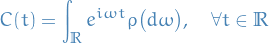
Correlation between two points of a random field or a random process:
to allow the possibility of an infinite number of points. In the discrete case this simply corresponds to the covariance matrix.
 denotes the Borel σ-algebra
- Partition

We write
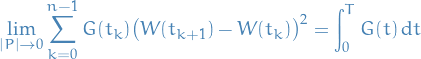
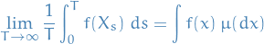
Whenever we write stochastic integrals as Riemann sums, e.g.
the limit is to be understood in the mean-square sense, i.e.
![\begin{equation*}
\mathbb{E} \Bigg[ \left| \int_{0}^{T} \dd{W}^2 \dd{w} - \bigg( \lim_{\left| P \right| \to 0} \sum_{k=0}^{n - 1} W^2(t_k) \big( W(t_{k + 1}) - W(t_k) \big) \bigg) \right|^2 \Bigg] \to 0
\end{equation*}](../../assets/latex/stochastic_differential_equations_2f41a4d7d8399bb2e7cfef31acb1c9ccdddb3dcf.png)
Definitions
A stochastic process  is called a either
- second-order stationary
- wide-sense stationary
- weakly stationary
if
- the first moment
![$\mathbb{E}[X_t]$](../../assets/latex/stochastic_differential_equations_8d9f7fa24439190f383b035eaa73b879837215fa.png) is constant
is constant - covariance function depends only on the difference

That is,
![\begin{equation*}
\mathbb{E}[X_t] = \mu, \quad \mathbb{E} \Big[ \big( X_t - \mu \big) \big( X_s - \mu \big) \Big] = C(t - s)
\end{equation*}](../../assets/latex/stochastic_differential_equations_5ea8e1b4c47525a0c8a992b042b08df9e7214354.png)
A stochastic process is called (strictly) stationary if all FDDs are invariant under time translation, i.e. for all  , for all times
  , and
, and  ,
,

for  such that
  , for every
  .
.
The autocorrelation function of a second-order stationary process enables us to associate a timescale to  , the correlation time
  :
:
![\begin{equation*}
\tau_{\text{cor}} = \frac{1}{C(0)} \int_{0}^{\infty} C(\tau) \ d \tau = \frac{1}{\mathbb{E}[X_0^2]} \int_{0}^{\infty} \mathbb{E}[X_{\tau} X_0] \ d \tau
\end{equation*}](../../assets/latex/stochastic_differential_equations_587f96c122fe76cd3bcdf77e7c449c337aba8116.png)
Martingale continuous processes
Let
![$\{ \mathscr{F}_t \}_{t \in [0, T]}$](../../assets/latex/stochastic_differential_equations_a4f2239efacde13545eb8c98a02a871f2c9a18a6.png) be a filtration defined on the probability space
be a filtration defined on the probability space 
![$\{ X_t \}_{t \in [0, T]}$](../../assets/latex/stochastic_differential_equations_8e67cdfcf601ca9e21ebb401175755d9c3b1fc84.png) be to
be to  , i.e. is measurable on , with
  .
.
We say is an martingale if
![\begin{equation*}
\mathbb{E} \big[ X_t \mid \mathscr{F}_s \big] = X_s, \quad \forall t \ge s
\end{equation*}](../../assets/latex/stochastic_differential_equations_0ca720db7443e47a4e9a323ec4b3ae03dc11d8ff.png)
Gaussian process
A 1D continuous-time Gaussian process is a stochastic process for which  , and all finite-dimensional distributions are Gaussians.
That is, for every finite dimensional vector

for some symmetric non-negative definite matrix  , for all and
  .
.
Theorems
Bochner's Theorem
Let  be a continuous positive definite function.
Then there exists a unique nonnegative measure  on
on  such that
  and
and
i.e. is the Fourier transform of the function .
Let be a second-order stationary process with autocorrelation function whose Fourier transform is  .
.
The measure is called the spectral measure of the process .
If the spectral measure is absolutely continuous wrt. the Lebesgue measure on with density  , i.e.

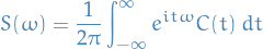
then the Fourier transform of the covariance function is called the spectral density of the process:
Ito vs. Stratonovich
- Purely matheamtical viewpoint: both Ito and Stratonovich calculi are correct
- Ito SDE is appropriate when continuous approximation of a discrete system is concerned
- Stratonovich SDE is appropriate when the idealization of a smooth real noise process is concerned
Benefits of Itô stochastic integral:
Benefits of Stratonovich stochastic integral:
- Leads to the standard Newton-Leibniz chain rule, in contrast to Itô integral which requires correction
- SDEs driven by noise with nonzero correlation time converge to the Stratonovich SDE, in the limit as the correlation time tends to 0
Practical considerations
- Rule of thumb:
- White noise is regarded as short-correlation approximation of a coloured noise → Stratonovich integral is natural
- "Expected" since the standard chain rule should work fro smooth noise with finite correlation
- White noise is regarded as short-correlation approximation of a coloured noise → Stratonovich integral is natural
Equivalence
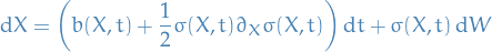
Suppose  solves the following Stratonovich SDE

then solves the Itô SDE:
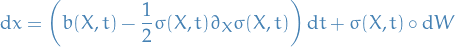
Suppose solves the Itô SDE:

then solves the Stratonovich SDE:
That is, letting 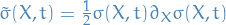 ,
,
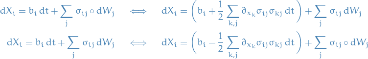
- Stratonovich → Itô:

- Itô → Stratonovich:

In the multidimensional case,
To show this we consider  staisfying the two SDEs

i.e. the satisfying the stochastic integrals

We have
Equivalently, we can write

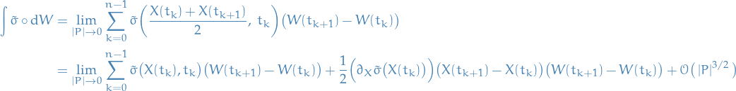
Assuming the  is smooth, we can then Taylor expand about
  and evaluate at
  :
:

Substituting this back into the Riemann series expression for the Stratonovich integral, we have
Using the fact that satisfies the Itô integral, we have

and that
we get

Thus, we have the identity

Matching the coefficients with the Itô integral satisfied by , we get

which gives us the conversion rules between the Stratonovich and Itô formulation!
Important to note the following though: here we have assumed that the  is smooth, i.e. infinitely differentiable and therefore locally Lipschitz. Therefore our proof only holds for this case.
I don't know if one can relax the smoothness constraint of  and still obtain conversion rules between the two formulations of the SDEs.
Stratonovich satisfies chain rule proven using conversion
For some function  , one can show that the Stratonovich formulation satisfies the standard chain rule by considering the Stratonovich SDE, converting to Itô, apply Itô's formula, and then converting back to Stratonovich SDE!
Variations of Brownian motion
Ornstein-Uhlenbeck process
Consider a mean-zero second-order stationary process with correlation function

We will write  , where
  .
.
The spectral density of this process is
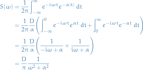
This is called a Cauchy or Lorentz distribution.
The correlation time is then
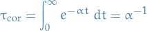
A real-valued Gaussian stationary process defiend on with correlation function as given above is called a Ornstein-Uhlenbeck process.
Look here to see the derivation of the Ornstein-Uhlenbeck process from it's Markov semigroup generator.
Fractional Brownian Motion
A (normalized) fractional Brownian motion  ,
,  , with Hurst parameter
  is a centered Gaussian process with continuous sample paths whose covariance is given by
![\begin{equation*}
\mathbb{E} \Big[ W_t^H W_s^H \Big] = \frac{1}{2} \Big( s^{2 H } + t^{2 H} - |t - s|^{2H} \Big)
\end{equation*}](../../assets/latex/stochastic_differential_equations_1969cb5b42b869ff1006e5965ecc49ae84cbd5d4.png)
Hence, the Hurst parameter controls:
- the correlations between the increments of fractional Brownian motion
- the regularity of the paths: they become smoother as
 increases.
A fractional Brownian motion has the following properties
- When
 , then
  becomes standard Brownian motion.
 We have
![\begin{equation*}
W_0^H = 0, \quad \mathbb{E} \Big[ \big(W_t^H\big)^2 \Big] = \left| t \right|^{2H}
\end{equation*}](../../assets/latex/stochastic_differential_equations_8c0d258d833885b8a8bd5c0580c7707f83dd0723.png)
It has stationary increments, and
![\begin{equation*}
\mathbb{E} \Big[ \big( W_t^H - W_s^H \big)^2 \Big] = \left| t- s \right|^{2H}
\end{equation*}](../../assets/latex/stochastic_differential_equations_e26c090c9022cb6663e364431a780f23248c560a.png)
It has the following self-similarity property:

where the equivalence is in law.
Karhunen-Loève Expansion
Notation
 where
where 
 be an orthonormal basis in
![$T = [0, 1]$](../../assets/latex/stochastic_differential_equations_23dced75d9a6ec5491322216c5886b4140c99f2e.png)
![$R(t, s) = \mathbb{E}[X_t X_s]$](../../assets/latex/stochastic_differential_equations_3b295160c01b3e49f52359d9016cb2bc6e61a130.png)
Stuff
Let ![$\mathscr{D} = [0, 1]$](../../assets/latex/stochastic_differential_equations_97cb4e38325c2c5a34d4a23d5f55de5c5e1b5204.png) .
.
Suppose
![\begin{equation*}
X_t(\omega) = \sum_{n=1}^{\infty} \xi_n(\omega) e_n(t), \quad t \in [0, 1]
\end{equation*}](../../assets/latex/stochastic_differential_equations_4a7cbe71aa0671bbd90019cc71a62e9ccd35b711.png)
We assume  are orthogonal or independent, and
![\begin{equation*}
\mathbb{E} \big[ \xi_n \xi_m \big] = \lambda_n \delta_{nm}
\end{equation*}](../../assets/latex/stochastic_differential_equations_e68b5cfb63a2da7f3d476bab49e1016d2c6ec9c5.png)
for some positive numbers  .
.
Then
![\begin{equation*}
\begin{split}
R(t, s) &= \mathbb{E}[X_t X_s] \\
&= \mathbb{E} \bigg( \sum_{k=1}^{\infty} \sum_{m=1}^{\infty} \xi_k e_k(t) \xi_m e_m(s) \bigg) \\
&= \sum_{k=1}^{\infty} \sum_{m=1}^{\infty} \mathbb{E}[\xi_k \xi_m] e_k(t) e_m(s) \\
&= \sum_{k=1}^{\infty} \lambda_k e_k(t) e_k(s)
\end{split}
\end{equation*}](../../assets/latex/stochastic_differential_equations_0f2c03172dac6146970a8f5b5085a3b654b1f040.png)
due to orthogonality of  and
and  for
for  .
.
Hence, for the expansion of  above, we need
  to be valid!
The above expression for  also implies
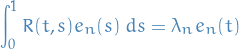
Hence, we also need the set  to be a set of eigenvalues and eigenvectors of the integral operator whose kernel is the correlation function of $Xt, i.e. need to study the operator
which we will now consider as an operator on ![$L^2 \big( [0, 1] \big)$](../../assets/latex/stochastic_differential_equations_e7126fcdebb9ebf5f71a45cf71db0142844a3b72.png) .
.
It's easy to see that  is self-adjoint and nonnegative in
  :
:

Furthermore, it is a compact operator, i.e. if  is a bounded sequence on , then
  has a convergent subsequence.
Spectral theorem for compact self-adjoint operators can be used to deduce that has a countable sequence of eigenvalues tending to  .
.
Furthermore, for every  , we can write
where  and
and  are the eigenfunctions of the operator corresponding to the non-zero eigenvalues and where the convergence is in
  , i.e. we can "project"
  onto the subspace spanned by eigenfunctions of .
Let ![$\{ X_t, t \in [0, 1] \}$](../../assets/latex/stochastic_differential_equations_1225f44e89bcd169ffb7b1eb3ed517c6bd62dd9a.png) be an process with zero mean and continuous correlation function .
be an process with zero mean and continuous correlation function .
Let  be the eigenvalues and eigenfunctions of the operator defined
Then
![\begin{equation*}
X_t = \sum_{n=1}^{\infty} \xi_n e_n(t), \quad t \in [0, 1]
\end{equation*}](../../assets/latex/stochastic_differential_equations_070cf4e790d3c037f3d71d457cd9e629ce3043c9.png)
where
![\begin{equation*}
\begin{split}
\xi_n &= \int_{0}^{1} X_t e_n(t) \ dt \\
\mathbb{E} \big[ \xi_n \big] &= 0 \\
\mathbb{E} \big[ \xi_n \xi_m \big] &= \lambda \delta_{n m}
\end{split}
\end{equation*}](../../assets/latex/stochastic_differential_equations_7b5cbc1b279426a8986865434401a8231ef5e979.png)
The series converges in to , uniformly in  !
!
Karhunen-Loève expansion of Brownian motion
- Correlation function of Brownian motion is
 .
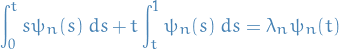
. Eigenvalue problem
 becomes
- Assume
 (since
  would imply ψn(t) = 0$)
 - Consider intial condition
 which gives
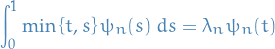
Can rewrite eigenvalue problem
Differentiatiate once

using FTC, we have
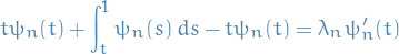
hence
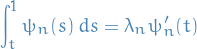
- Obtain second BC by observing
 (since LHS in the above is clearly 0)
 Second differentiation
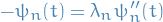
Thus, the eigenvalues and eigenfunctions of the integral operator whose kernel is the covariance function of Brownian motion can be obtained as solutions to the Sturm-Lioville problem

Eigenvalues and (normalized) eigenfunctions are then given by
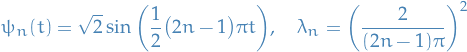
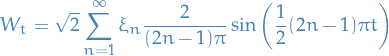
Karhunen-Loève expansion of Brownian motion on
![$[0, 1]$](../../assets/latex/stochastic_differential_equations_68c8fa38d960e53d4308cbf1e65d04c66a554817.png) is then
is then
Diffusion Processes
Notation
 and state space
  denotes the
 Markov Processes and the Chapman-Kolmogorov Equation
We define the σ-algebra generated by  , denoted
  , to be the smallest σ-algebra s.t. the family of mappings
  is a stochastic process with
- sample space
- state space

- Idea: encode all past information about a stochastic process into an appropriate collection of σ-algebras
Let denote a probability space.
Consider stochastic process  with
with  and state space .
A filtration on  is a nondecreasing family
  of sub-σ-algebras of
  :
:

We set
Note that  is a possibility.
The filtration generated by or natural filtration of the stochastic process is

A filtration  is generated by events of the form

with  and
and  .
.
Let be a stochastic process defined on a probability space with values in  , and let be the filtration generated by
  .
.
Then  is a Markov process if

for all  with
with  , and
, and  .
.
Equivalently, it's a Markov process if

for  and with
  .
.
Chapman-Kolmogorov Equation
The transition function  for fixed
  is a probability measure on with
It is  measurable in
  , for fixed
  , and satisfies the Chapman-Kolmogorov equation
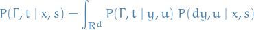
for all

 with
with 
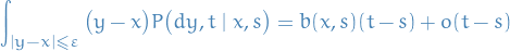
Assuming that  , we can write
![\begin{equation*}
P(\Gamma, t \mid x, s ) = \mathbb{P} \big[ X_t \in \Gamma \mid X_s = x \big]
\end{equation*}](../../assets/latex/stochastic_differential_equations_a2caf2b6f9a9de649a064e6bcf54c04f6f39838d.png)
since ![$\mathbb{P} \big[ X_t \in \Gamma \mid \mathscr{F}_s^X \big] = \mathbb{P} \big[ X_t \in \Gamma \mid X_s \big]$](../../assets/latex/stochastic_differential_equations_eac94ebb86be9c955d319e80319525a5e83f2e6c.png) .
.
In words, the Chapman-Kolmogorov equation tells us that for a Markov process, the transition from at time  to the set
  at time can be done in two steps:
- System moves from to
 at some intermediate step
- Moves from to at time
Generator of a Markov Process
Chapman-Kolmogorov equation suggests that a time-homogenous Markov process can be described through a semigroup of operators, i.e. a one-parameter family of linear operators with the properties

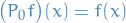
Let  be the transition function of a homogenous Markov process and let
  , and define the operator
![\begin{equation*}
\big( P_t f \big)(x) := \mathbb{E} \Big[ f(X_t) \mid X_0 = x \Big] = \int_{\mathbb{R}^d}^{} f(y) \ P(t, x, dy)
\end{equation*}](../../assets/latex/stochastic_differential_equations_650c4cf9438bd1c8253e889eaba8a58ce2cf59af.png)
Linear operator with
which means that  , and
, and

i.e.  .
.
We can study properties of time-homogenous Markov process by studying properties of the Markov semigroup  .
.
This is an example of a strongly continuous semigroup.
Let  be set of all
  such that the limit
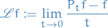
exists.
The operator  is called the (infinitesimal) generator of the operator semigroup
- Also referred to as the generator of the Markov process
This is an example of a (infinitesimal) generator of a strongly continuous semigroup.
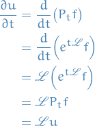
The semigroup property of the generator of the Markov process implies that we can write

Furthermore, consider function
![\begin{equation*}
u(x, t) = \big( P_t f \big)(x) = \mathbb{E} \Big[ f(X_t) \mid X_0 = x \Big]
\end{equation*}](../../assets/latex/stochastic_differential_equations_f32e574b9643a44a3640f02130ba9d0f43bf51ac.png)
Compute time-derivative
And we also have

Consequently,  satisfies the IVP
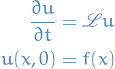
which defines the backward Kolmogorov equation.
This equation governs the evolution of the expectation of an observalbe .
Example: Brownian motion 1D
- Transition function for Brownian motion is given by the fundamental solution to the heat equation in 1D
Corresponding Markov semigroup is the heat semigroup
- Generator of the 1D Brownian motion is then the 1D Laplacian

The backward Kolmorogov equation is then the heat equation
Adjoint semigroup
Let be a Markov semigroup, which then acts on  .
.
The adjoint semigroup  acts on probability measures:
The image of a probability measure  under is again a probability measure.
The operators and are adjoint in the sense:
We can write

where  is the adjoint of the generator of the Markov process:
Let be a Markov process with generator with  , and let denote the adjoint Markov semigroup.
We define

This is the law of the Markov process. This follows the equation
Assuming that the initial distribution and the law of the process  each have a density wrt. Lebesgue measure, denoted
  and
and  , respectively, the law becomes
which defines the forward Kolmorogov equation.
"Simple" forward Kolmogorov equation
Consider SDE

Since
is Markovian, its evoluation can be characterised by a transition probability  :
:
![\begin{equation*}
\mathbb{P} \Big( X(t) \in [x, x + \dd{t}] : X(s) = y \Big) = p(x, t \mid y, s) \dd{x}
\end{equation*}](../../assets/latex/stochastic_differential_equations_df4f6b62ca1e95add6d6557ce08703c3e1d270b6.png)
Consider
 , then
![\begin{equation*}
\dd{\Big( f \big( X(u) \big) \Big)} = \partial_x f \Big( X(u) \Big) \Big[ b \big( X(u), u \big) \dd{u} + \sigma \big( X(u), u \big) \dd{W} \Big] + \frac{1}{2} \partial_{xx} f \Big( X(u) \Big) \sigma^2 \Big( X(u), u \Big) \dd{u}
\end{equation*}](../../assets/latex/stochastic_differential_equations_b96cbc3de78139e9888f72b2385039877196203a.png)
Ergodic Markov Processes
Using the adjoint Markov semigroup, we can define the invariant measure as a probability measure that is invariant under time evolution of , i.e. a fixed point of the semigroup :

A Markov process is said to be ergodic if and only if there exists a unique invariant measure .
We say the process is ergodic wrt. the measure .
Furthermore, if we consider a Markov process in with generator  and Markov semigroup , we say that is ergodic provided that is a simple eigenvalue of , i.e.

has only constant solutions.
Thus, we can study the ergodic properties of a Markov process by studying the null space of the its generator.
We can then obtain an equation for the invariant measure in terms of the adjoint of the generator.
Assume that has a density wrt. the Lebesgue measure. Then
by definition of the generator of the adjoint semigroup.
Furthermore, the long-time average of an observable converges to the equilibrium expectation wrt. the invariant measure
1D Ornstein-Uhlenbeck process and its generator
The 1D Ornstein-Uhlenbeck process is an ergodic Markov process with generator
The null-space of comprises of constants in , hence it is an ergodic Markov process.
In order to find the invariant measure, we need to solve the stationary Fokker-Planck equation:
Which clearly require that we have an expression for . We have , so
![\begin{equation*}
\begin{split}
\int_{\mathbb{R}}^{} \mathscr{L}f \ h \ dx &= \int_{\mathbb{R}}^{} \bigg[ \bigg( - \alpha x \frac{df}{dx} \bigg) + \bigg( D \frac{d^2 f}{dx^2} \bigg) \bigg] \ dx \\
&= \int_{\mathbb{R}}^{} \Big[ f \partia_x \big( \alpha x h \big) + f \big( D \partial_x^2 h \big) \Big] \ dx \\
&=: \int_{\mathbb{R}}^{} f \mathscr{L}^* h \ dx
\end{split}
\end{equation*}](../../assets/latex/stochastic_differential_equations_e09dc286790d97633168df255296229a360c69b5.png)
Thus,
Substituting this expression for back into the equation above, we get
which is just a Gaussian measure!
Observe that in the above expression, the stuff on LHS before  corresponds to
  in the equation we solved for .
If  (i.e. distributed according to the invariant measure derived above), then is a mean-zero Gaussian second-order stationary process on
  with correlation function
and spectral density
as seen before!
Furthermore, Ornstein-Uhlenbeck process is the only real-valued mean-zero Gaussian second-order stationary Markov process with continuous paths defined on .
Diffusion Processes
Notation
 means depends on terms dominated by linearity in
Stuff
A Markov process consists of three parts:
- a drift
- a random part
- a jump process
A diffusion process is a Markov process with no jumps.
A Markov process in with transition function is called a diffusion process if the following conditions are satisfied:
(Continuity) For every
and  ,
,
uniformly over

( Drift coefficient ) There exists a function
 s.t. for every and every ,
uniformly over
.
( Diffusion coefficient ) There exists a function
 s.t. for every and every ,

uniformly over
.
Important: above we've truncated the domain of integration, since we do not know whether the first and second moments of are finite. If we assume that there exists  such that
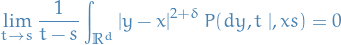
then we can extend integration over all of and use expectations in the definition of the drift and the diffusion coefficient , i.e. the drift:
![\begin{equation*}
\lim_{t \to s} \mathbb{E} \bigg[ \frac{X_t - X_s}{t - s} \bigg| X_s = x \bigg] = b(x, s)
\end{equation*}](../../assets/latex/stochastic_differential_equations_1a3b70c34987a635cd59988bc20315b883cf348e.png)
and diffusion coefficient:
![\begin{equation*}
\lim_{t \to s} \mathbb{E} \bigg[ \frac{\left| X_t - X_s \right|^2}{t - s} \bigg| X_s = x \bigg] = \Sigma(x, s)
\end{equation*}](../../assets/latex/stochastic_differential_equations_7b7e831fbb6901407e7a79fa490c7e5b5ada2474.png)
Backward Kolmogorov Equation
Let  , and let
![\begin{equation*}
u(x, s) := \mathbb{E} \Big[ f(X_t) \mid X_s = x \Big] = \int_{}^{} f(y) \ P(dy, t \mid x, s)
\end{equation*}](../../assets/latex/stochastic_differential_equations_3fcabfeb4cba60a7f3d3bc9bcd9c38a8e8afb88c.png)
with fixed .
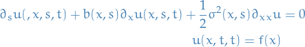
Assume, furthermore, that the functions and are smooth in both and .
Then  solves the final value problem
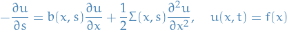
for ![$s \in [0, t]$](../../assets/latex/stochastic_differential_equations_a01cab2a0ca7fa7a95b9372d9031b49f2bd03f76.png) .
.
For a proof, see Thm 2.1 in pavliotis2014stochastic. It's clever usage of the Chapman-Kolmogorov equation and Taylor's theorem.
For a time-homogenous diffusion process, where the drift and the diffusion coefficents are independent of time:

we can rewrite the final value problem defined by the backward Kolmogorov equation as an initial value problem.
Let  , and introduce
  . Then,
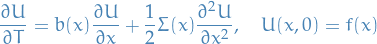
Further, we can let  , therefore

where
![\begin{equation*}
u(x, t) = \mathbb{E} \Big[ f(X_t) \mid X_0 = x \Big]
\end{equation*}](../../assets/latex/stochastic_differential_equations_453e5e2378adb55ddec75660c12a82c4813b1c20.png)
is the solution to the IVP.
Forward Kolmorogov Equation
Assume that the conditions of a diffusion process are satisfied, and that the following are smooth functions of and :


Then the transition probability density is the solution to the IVP

For proof, see Thm 2.2 in pavliotis2014stochastic. It's clever usage of Chapman-Kolmogorov equation.
Solving SDEs
This section is meant to give an overview over the calculus of SDEs and tips & tricks for solving them, both analytically and numerically. Therefore this section might be echoing other sections quite a bit, but in a more compact manner most useful for performing actual computations.
Notation
Analytically
"Differential calculus"
 =
= 
 for all
If multivariate case, typically one will assume white noise to be indep.:

Suppose we have some SDE for
, i.e. some expression for  .
Change of variables
.
Change of variables  then from Itô's lemma we have
where
 is computed by straight forward substitution by expression for and using the "properties" of
Letting
 and
and  in Itô's lemma we get
Letting
and 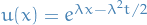 , then Itô's lemma gets us
Hence
 satisfies the geometric Brownian motion SDE.
Numerically
Numerical SDEs
Notation

We willl consider an SDE with the exact solution

Convergence
The strong error is defined
![\begin{equation*}
e_{\Delta t}^{\text{strong}} := \sup_{0 \le t_n \le T} \mathbb{E} \big[ \left| X_n - X(t_n) \right| \big]
\end{equation*}](../../assets/latex/stochastic_differential_equations_68efec6daabf5c6f11a5e4ad62da5dce62abc462.png)
We say a method converges strongly if
We say the method has strong order  if
if

Basically, this notion of convergence talks about how "accurately" paths are followed.
Error on individual path level
Euler-Maryuama has
![\begin{equation*}
\mathbb{E} \big[ \left| X_n - X(t_n) \right| \big] \le K \Delta t ^{\frac{1}{2}}
\end{equation*}](../../assets/latex/stochastic_differential_equations_44c28c2bdca36e182b6cb2ac704fc867961d9520.png)
Markov inequality says
![\begin{equation*}
\mathbb{P} \big( \left| X \right| > \alpha \big) \le \frac{\mathbb{E} \big[ \left| X \right| \big]}{\alpha}
\end{equation*}](../../assets/latex/stochastic_differential_equations_1d59e14e6a22a2a668a50fd9912b2fbb8d39ea49.png)
for any
 .
.
Let
 gives
gives
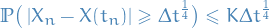
i.e.

- That is, along any path the error is small with high probability

 .
.
Stochastic Taylor Expansion
Deterministic ODEs
Consider
For some function, we then write

where
and the
 is due to the above
- This looks quite a bit like the numerical quadrature rule, dunnit kid?!
- Because it is!
We can then do the same for
 :
:
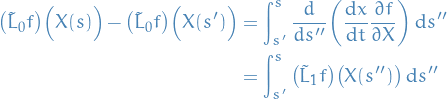
where
![\begin{equation*}
\big( \tilde{L}_1 f \big) \big( X(t) \big) = \dv{}{t} \bigg( \dv{x}{t} \frac{\partial f}{\partial x} \bigg) = \dv[2]{x}{t} \frac{\partial f}{\partial x} + \bigg( \dv{x}{t} \bigg)^2 \pdv[2]{f}{x}
\end{equation*}](../../assets/latex/stochastic_differential_equations_5f1ba462ce108266e939340b4242c04356adf851.png)
- We can then substitute this back into the original integral, and so on, to obtain higher and higher order
- This is basically just performing a Taylor expansion around a point wrt. the stepsize

- For an example of this being used in a "standard" way; see how we proved Euler's method for ODEs
- Reason for using integrals rather than the the "standard" Taylor expansion to motivate the stochastic way of doing this, where we cannot properly talk about taking derivatives
Stochastic
- Idea: extend the "Taylor expansion method" of obtaining higher order numerical methods for ODEs to SDEs
Consider
Satisfies the Itô integral

- Can do the same as before for each of the integral terms:
 :
:
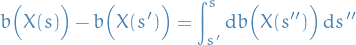
but in this stochastic case, we have to use Itô's formula
so
![\begin{equation*}
b \Big( X(s) \Big) - b \Big( X(s') \Big) = \frac{1}{2} \int_{s'}^{s} \pdv[2]{b}{X} \dd{s''} + \int_{s'}^{s} \pdv{b}{X} \dd{X(s'')}
\end{equation*}](../../assets/latex/stochastic_differential_equations_9952697df75c5a4e9be4c5932214801fa5c663d1.png)
- :
![\begin{equation*}
\sigma \Big( X(s) \Big) - \sigma \Big( X(s') \Big) = \frac{1}{2} \int_{s'}^{s} \pdv[2]{\sigma}{X} \dd{s''} + \int_{s'}^{s} \pdv{\sigma}{X} \dd{X(s'')}
\end{equation*}](../../assets/latex/stochastic_differential_equations_2853365c0d2abf6ff232b39e764a79d466e1ee33.png)
Then we can substitute these expressions into our original expression for
 :
:
![\begin{equation*}
\begin{split}
X(t + h) - X(t) &= \int_{t}^{t + h} \bigg[ b \big( X(s') \big) + \frac{1}{2} \int_{s'}^{s} \pdv[2]{b}{X} \dd{s''} + \int_{s'}^{s} \pdv{b}{X} \dd{X(s'')} \bigg] \dd{s} \\
& \quad + \int_{t}^{t + h} \bigg[ \sigma \Big( X(s') \Big) + \frac{1}{2} \int_{s'}^{s} \pdv[2]{\sigma}{X} \dd{s''} + \int_{s'}^{s} \pdv{\sigma}{X} \dd{X(s'')} \bigg] \dd{W(s)}
\end{split}
\end{equation*}](../../assets/latex/stochastic_differential_equations_50aa343322e20485f21a70fb9ad0a279ad24f093.png)
Observe that we can bring the terms
 and
and  out of the integrals:
![\begin{equation*}
\begin{split}
X(t + h) - X(t) &= b \big( X(s') \big) \underbrace{\int_{t}^{t + h} \dd{s}}_{= h} + \int_{t}^{t + h} \bigg[ \frac{1}{2} \int_{s'}^{s} \pdv[2]{b}{x} \dd{s''} + \int_{s'}^{s} \pdv{b}{X} \dd{X(s'')} \bigg] \dd{s} \\
& \quad + \sigma \big( X(s') \big) \underbrace{\int_{t}^{t + h} \dd{W(s)}}_{= W(t + h) - W(t) = \Delta W} \\
& \quad + \int_{t}^{t + h} \bigg[ \frac{1}{2} \int_{s'}^{s} \pdv[2]{\sigma}{X} \dd{s''} + \int_{s'}^{s} \pdv{\sigma}{X} \dd{X(s'')} \bigg] \dd{W(s)} \\
&= b \big( X(s') \big) h + \int_{t}^{t + h} \bigg[ \frac{1}{2} \int_{s'}^{s} \pdv[2]{b}{x} \dd{s''} + \int_{s'}^{s} \pdv{b}{X} \dd{X(s'')} \bigg] \dd{s} \\
& \quad + \sigma \big( X(s') \big) \Delta W + \int_{t}^{t + h} \bigg[ \frac{1}{2} \int_{s'}^{s} \pdv[2]{\sigma}{X} \dd{s''} + \int_{s'}^{s} \pdv{\sigma}{X} \dd{X(s'')} \bigg] \dd{W(s)}
\end{split}
\end{equation*}](../../assets/latex/stochastic_differential_equations_e47f65fbc312ada51b9c299b272a10858dce4176.png)
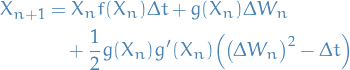
- Observe that the two terms that we just brought out of the integrals define the Euler-Maruyama method!!
- Bloody dope, ain't it?
Connections between PDEs and SDEs
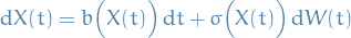
Suppose we have an SDE of the form

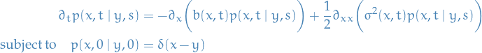
Forward Kolmogorov / Fokker-Plank equation
Then the Fokker-Planck / Forward Kolmogorov equation is given by the following ODE:
Derivation of Forward Kolmogorov
Suppose we have an SDE of the form
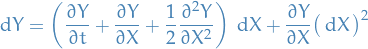
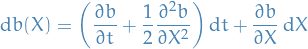
Consider twice differentiable function  , then Itô's formula gives us
![\begin{equation*}
\begin{split}
\dd{f \big( X(t) \big)} &= \partial_t f \big( X(t) \big) \dd{t} + \partial_x f \big( X(t) \big) \dd{X(t)} + \frac{1}{2} \partial_{xx} f \big( X(t) \big) \big( \dd{X(t)} \big)^2 \\
&= \partial_x f \big( X(t) \big) \Big[ b \big( X(t), t \big) \dd{t} + \sigma^2 \big( X(t), t \big) \dd{W(t)} \Big] + \frac{1}{2} \partial_{xx} f \big( X(t) \big) \dd{t}
\end{split}
\end{equation*}](../../assets/latex/stochastic_differential_equations_5c66131e332963d70a943a25bd03efe68d3142d9.png)
which then satisfies the Itô integral
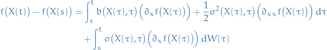
Taking the (conditional) expectation, the last term vanish, so LHS becomes
![\begin{equation*}
\begin{split}
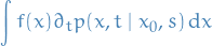
\mathbb{E} \Big[ f \big( X(t) \big) - f \big( X(s) \big) \mid X(s) = x_0 \Big] &= \mathbb{E} \Big[ f \big( X(t) \big) \mid X(s) = x_0 \Big] - f(x_0) \\
&= \bigg( \int_{}^{} f( x ) p(x, t \mid x_0, s) \dd{x} \bigg) - f(x_0)
\end{split}
\end{equation*}](../../assets/latex/stochastic_differential_equations_7af9f83c50a8d955ceaef50bacea3cc649c1d9fd.png)
and RHS
![\begin{equation*}
\begin{split}
& \mathbb{E} \Bigg[ \int_{s}^{t} b \big( X(\tau), \tau \big) \Big( \partial_x f \big( X(\tau) \big) \Big) + \frac{1}{2} \sigma^2 \big( X(\tau), \tau \big) \Big( \partial_{xx} f \big( X(\tau) \big) \Big) \dd{\tau} \ \bigg| \ X(s) = x_0 \Bigg] \\
= \quad & \int_{}^{} \bigg( \int_{s}^{t} p(x, \tau \mid x_0, s) \bigg[ b \big( x, \tau \big) \Big( \partial_x f(x) \Big) + \frac{1}{2} \sigma^2 \big( x, \tau \big) \Big( \partial_{xx} f (x) \Big) \bigg] \dd{\tau} \bigg) \dd{x}
\end{split}
\end{equation*}](../../assets/latex/stochastic_differential_equations_221076c0f59c76cc297abf9cdd940b1dc1c3c055.png)
Taking the derivative wrt. , LHS becomes
and RHS
![\begin{equation*}
\int p(x, t \mid x_0, s) \bigg[ b \big( x, t \big) \Big( \partial_x f(x) \Big) + \frac{1}{2} \sigma^2 \big( x, t \big) \Big( \partial_{xx} f (x) \Big) \bigg] \dd{x}
\end{equation*}](../../assets/latex/stochastic_differential_equations_79869131775111ee7c958dd3802537ac57499d76.png)
The following is actually quite similar to what we do in variational calculus for our variations!
Here we first use the standard "integration by parts to get rather than derivatives of ", and then we make use of the Fundamental Lemma of the Calculus of Variations!
Using integration by parts in the above equation for RHS, we have
![\begin{equation*}
\int \bigg[ - \partial_x \Big( p(x, t \mid x_0, s) b(x, t) \Big) + \frac{1}{2} \partial_{xx} \Big( p(x, t \mid x_0, s) \sigma^2(x, t) \Big) \bigg] f(x) \dd{x}
\end{equation*}](../../assets/latex/stochastic_differential_equations_33c80d5bb4ce09dc3587f5afdab2ea378df16f48.png)
where we have assumed that we do not pick up any extra terms (i.e. the functions vanish at the boundaries). Hence,
![\begin{equation*}
\int f(x) \Big( \partial_t p(x, t \mid x_0, s) \Big) \dd{x} = \int \bigg[ - \partial_x \Big( p(x, t \mid x_0, s) b(x, t) \Big) + \frac{1}{2} \partial_{xx} \Big( p(x, t \mid x_0, s) \sigma^2(x, t) \Big) \bigg] f(x) \dd{x}
\end{equation*}](../../assets/latex/stochastic_differential_equations_b9c93801fa9da8ed2e26ae06d732730b2a68c597.png)
Since this holds for all  , by the Fundamental Lemma of Calculus of Variations, we need

which is the Fokker-Planck equation, as wanted!
Assumptions
In the derivation above we assumed that the non-integral terms vanished when we performed integration by parts. This is really assuming one of the following:
- Boundary conditions at
 :
:  as
as 
- Absorbing boundary conditions: where we assume that
 for
for  (the boundary of the domain
  )
) - Reflecting boundary conditions: this really refers to the fact that multidimensional variations vanish has vanishing divergence at the boundary. See multidimensional Euler-Lagrange and the surrounding subjects.
Backward equation
And the Backward Kolmogorov equation:
where
![\begin{equation*}
u(x, s, t) = \big( P_t f \big)(x) = \mathbb{E} \Big[ f \big( X(t) \big) \mid X(s) = x \Big], \quad t \ge s
\end{equation*}](../../assets/latex/stochastic_differential_equations_c5f7341f119d84d5d47e34f5b4bc0505f5b7085b.png)
Here we've used  defined as
![\begin{equation*}
\big( P_t f \big)(x) = \mathbb{E} \Big[ f \big( X(t) \big) \mid X(s) = x \Big]
\end{equation*}](../../assets/latex/stochastic_differential_equations_cb500821636d36ac05c4726b19225eced9685e83.png)
rather than
![\begin{equation*}
\big( P_t f \big)(x) = \mathbb{E} \Big[ f \big( X(t) \big) \mid X(0) = x \Big]
\end{equation*}](../../assets/latex/stochastic_differential_equations_b1926b7478d755d25ab8c049fc27c78953ad4314.png)
as defined before.
I do this to stay somewhat consistent with notes in the course (though there the operator is not mentioned explicitly), but I think using would simplify things without loss of generality (could just define the equations using  and
and  , and substitute back when finished).
Furthermore, if  and
and  , i.e. time-independent (autonomous system), then

in which case the Forward Kolmogorov equation becomes
where we've used the fact that in this case  .
.
Notation of generator of the Markov process and its adjoint
In the notation of the generator of the Markov process we have
![\begin{equation*}
\begin{split}
\mathcal{L} u &= b(x, t) \pdv{u}{x} + \frac{1}{2} \sigma^2(x, t) \pdv[2]{u}{t} \\
\mathcal{L}^* \rho &= - \pdv{}{x} \Big( b(x, t) \rho \Big) + \frac{1}{2} \pdv[2]{}{x} \Big( \sigma^2(x, t) \rho \Big)
\end{split}
\end{equation*}](../../assets/latex/stochastic_differential_equations_aad09fdd9f274ca752316028b16d9df7ece8cc8e.png)
TODO Introduction to Stochastic Differential Equations
Notation
 indicates the dependence on the initial condition
  .
.Stopping time

Motivation
We will consider stochastic differential equations of the form

or, equivalently, componentwise,
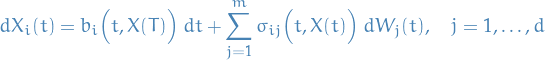
which is really just notation for
Need to define stochastic integral
for sufficiently large class of functions.
- Since Brownian motion is not of bounded variation → Riemann-Stieltjes integral cannot be defined in a unique way
Itô and Stratonovich Stochastic Integrals
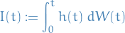
Let
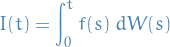
where  is a Brownian motion and
 ![$t \in [0, T]$](../../assets/latex/stochastic_differential_equations_a2d5fb401a604a95248d145edaa967973c136562.png) , such that
, such that
![\begin{equation*}
\mathbb{E} \bigg[ \int_{0}^{T} f(s)^2 \ ds \bigg] < \infty
\end{equation*}](../../assets/latex/stochastic_differential_equations_6923cd2757f7af08ca383a9c451640fd55daedc7.png)
Integrand is a stochastic process whose randomness depends on , and in particular, that is adapted to the filtration generated by the Brownian motion , i.e. that is an  function for all .
Basically means that the integrand depends only on the past history of the Brownian motion wrt. which we are integrating.
We then define the stochastic integral  as the
  (
( is the underlying probability space) limit of the Riemann sum approximation
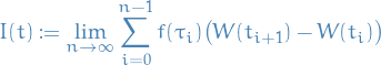
where
 where
where  is s.t.
![$\lambda \in [0, 1]$](../../assets/latex/stochastic_differential_equations_7cd670af2080b3c73aac2cd9f356000145119694.png)
increments

What we are really saying here is that (which itself is a random variable, i.e. a measurable function on the probability space  ) is the limit of the Riemann sum in a mean-square sense, i.e. converges in !
![\begin{equation*}
\begin{split}
& \mathbb{E} \Bigg[ \left| I(t) - \lim_{n \to \infty} \sum_{i=0}^{n - 1} f(\tau_i) \big( W(t_{i + 1}) - W(t_i) \big) \right|^2 \Bigg] \\
& \quad = \int_{\Omega} \left| I(t) - \lim_{n \to \infty} \sum_{i=0}^{n - 1} f(\tau_i) \big( W(t_{i + 1}) - W(t_i) \big) \right|^2 \dd{P} \\
& \quad = 0
\end{split}
\end{equation*}](../../assets/latex/stochastic_differential_equations_5ab3f253cbbe4e45691de5ac5b088d29ad66f5bb.png)
I found this Stackexchange answer to be very informative regarding the use of Riemann sums to define the stochastic integral.
Let be a stochastic integral.
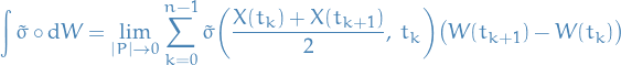
The Stratonovich stochastic integral is when  , i.e.
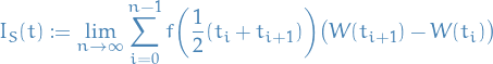
We will often use the notation
to denote the Stratonovich stochastic integral.
Observe that  does not satisfy the Martingale property, since we are taking the midpoint in
 ![$[t_k, t_{k + 1}]$](../../assets/latex/stochastic_differential_equations_cb683a2b95e8f305f3febcbd22819f76e61ab375.png) , therefore
, therefore  is correlated with !
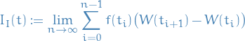
Itô instead uses the Martingale property by evaluating at the start point of the integral, and thus there is no auto correlation between the  and
and  , making it much easier to work with.
Suppose that there exist  s.t.
s.t.
![\begin{equation*}
\mathbb{E} \Big[ \big( f(t) - f(s) \big)^2 \Big] \le C \left| t - s \right|^{1 + \delta}, \quad 0 \le s, t \le T
\end{equation*}](../../assets/latex/stochastic_differential_equations_4aee2794d002a4533abd2b23d204ba3e05dc398e.png)
Then the Riemann sum approximation for the stochastic integral converges in  to the same value for all .
From the definition of a stochastic integral, we can make sense of a "noise differential equation", or a stochastic differential equation

with  being white noise.
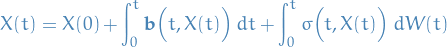
The solution then satisfies the integral equation
which motivates the notation

since, in a way,
(sometimes you will actually see the Brownian motion (this definition for example) defined in this manner, e.g. lototsky2017stochastic)
Properties of Itô stochastic integral
Itô isometry
Let be a Itô stochastic integral, then
![\begin{equation*}
\mathbb{E} \bigg[ \bigg( \int_{0}^{T} f(t) \ d W(t) \bigg)^2 \bigg] = \int_{0}^{T} \mathbb{E} \big[ \left| f(t) \right|^2 \big] \ dt
\end{equation*}](../../assets/latex/stochastic_differential_equations_fb938d7ae516ef815408e6ba427edacf5570c4b4.png)
From which it follows that for any square-integrable functions 
![\begin{equation*}
\mathbb{E} \bigg[ \bigg( \int_{0}^{T} h(t) \ d W(t) \int_{0}^{T} g(s) \ d W(s) \bigg) \bigg] = \mathbb{E} \bigg[ \int_{0}^{T} h(t) g(t) \ dt \bigg]
\end{equation*}](../../assets/latex/stochastic_differential_equations_4f628438f07e2d293292d9459a7513d58a6020e0.png)
![\begin{equation*}
\begin{split}
\mathbb{E} \bigg[ \bigg( \int_{0}^{T} f(t) + h(t) \ d W(t) \bigg)^2 \bigg]
&= \mathbb{E} \bigg[ \bigg( \int_{0}^{T} f(t) \ d W(t) \bigg)^2 + \bigg( \int_{0}^{T} h(t) \ d W(t) \bigg)^2 \\
& \qquad \quad + 2 \bigg( \int_{0}^{T} f(t) h(t) \ d W(t) \bigg) \bigg] \\
&= \int_{0}^{T} \mathbb{E} \big[ \left| f(t) \right|^2 \big] \ dt + \int_{0}^{T} \mathbb{E} \big[ \left| h(t) \right|^2 \big] \ d W(t) \\
& \qquad \quad + 2 \ \mathbb{E} \bigg[ \bigg( \int_{0}^{T} f(t) h(t) \ d W(t) \bigg) \bigg]
\end{split}
\end{equation*}](../../assets/latex/stochastic_differential_equations_e91e0d2442c044d62e44b072b27a636058360589.png)
but we also know that
![\begin{equation*}
\begin{split}
\mathbb{E} \bigg[ \bigg( \int_{0}^{T} f(t) + h(t) \ d W(t) \bigg)^2 \bigg] &= \int_{0}^{T} \mathbb{E} \big[ \left| f(t) + h(t) \right|^2 \big] \ dt \\
&= \int_{0}^{T} \mathbb{E} \big[ \left| f(t) \right|^2 \big] \ dt + \int_{0}^{T} \mathbb{E} \big[ \left| h(t) \right|^2 \big] \\
& \qquad + 2 \int_{0}^{T} \mathbb{E} \big[ \left| f(t) h(t) \right| \big] \ dt
\end{split}
\end{equation*}](../../assets/latex/stochastic_differential_equations_9f879b6173fae42516b10510f2ac63847b128e62.png)
Comparing with the equation above, we see that
![\begin{equation*}
\mathbb{E} \bigg[ \bigg( \int_{0}^{T} f(t) h(t) \ d W(t) \bigg) \bigg] = \mathbb{E} \bigg[ \int_{0}^{T} f(t) h(t) \ dt \bigg]
\end{equation*}](../../assets/latex/stochastic_differential_equations_c881fd770e7c6abd5046b9e697d22b2f0fe23aaa.png)
WHAT HAPPENED TO THE ABSOLUTE VALUE MATE?! Well, in the case where we are working with real functions, the Itô isometry is satisfied for  since it's equal to
  , which would give us the above expression.
Martingale
For Itô stochastic integral we have
![\begin{equation*}
\mathbb{E} \bigg[ \int_{0}^{t} f(s) \ d W(s) \bigg] = 0
\end{equation*}](../../assets/latex/stochastic_differential_equations_e0b6cca05557ad2516584ec171f972e15a79ddff.png)
and
![\begin{equation*}
\mathbb{E} \bigg[ \int_{0}^{t} f(\ell) \ d W(\ell) \ \bigg| \ \mathscr{F}_s \bigg] = \int_{0}^{s} f(\ell) \ d W(\ell), \quad \forall t \ge s
\end{equation*}](../../assets/latex/stochastic_differential_equations_8fbada2b8f8a2d42a36cf0e9d18f4182125d905d.png)
where  denotes the filtration generated by
  , hence the Itô integral is martingale.
The quadratic variation of this martingale is
Solutions of SDEs
Consider SDEs of the form

where
![$\mathbf{b}: [0, T] \times \mathbb{R}^d \to \mathbb{R}^d$](../../assets/latex/stochastic_differential_equations_9bfe6b358b9e1fbfe189485a8a952ec774c9685c.png)
![$\boldsymbol{\sigma}: [0, T] \times \mathbb{R}^{d} \to \mathbb{R}^{d \times m}$](../../assets/latex/stochastic_differential_equations_fd83ecd1f5fc746d9bf2c757c21fa4c09ee5dd6c.png)
A process with continuous paths defined on the probability space  is called a strong solution to the SDE if:
- is a.s. continuous and adapted to the filtration
 and
and  a.s.
a.s.For every
, the stochastic integral equation
Let
satisfy the following conditions
There exists positive constant
 s.t. for all and

For all
 and ,
and ,

Furthermore, suppose that the initial condition is a random variable independent of the Brownian motion  with
with
![\begin{equation*}
\mathbb{E} \big[ \norm{x}^2 \big] < \infty
\end{equation*}](../../assets/latex/stochastic_differential_equations_2d27c751e7fca7eb3452d0a396a0a7389e26a3d0.png)
Then the SDE
has a unique strong solution with
![\begin{equation*}
\mathbb{E} \bigg[ \int_{0}^{t} \norm{X_s}^2 \ ds \bigg] < \infty, \quad \forall t \in [0, T]
\end{equation*}](../../assets/latex/stochastic_differential_equations_808b76e7e8694667082a16a47df91937c9f2dc5b.png)
where by unique we mean
![\begin{equation*}
X_t \overset{a.s.}{=} Y_t, \quad \forall t \in [0, T]
\end{equation*}](../../assets/latex/stochastic_differential_equations_c97999eabdc7c14abb1b33bea29438998a705a25.png)
for all possible solutions and  .
.
Itô's Formula
Notation
Stuff
Consider Itô SDE

- is a diffusion process with drift
 and diffusion matrix
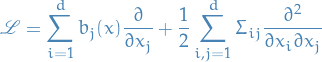
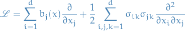
The generator
is then defined as
Assume that the conditions used in thm:unique-strong-solution hold.
Let be the solution of

and let ![$V \in C^{1, 2} \big( [0, T] \times \mathbb{R}^d \big)$](../../assets/latex/stochastic_differential_equations_fed8860d87af42a04708c72ec34b91d85f59a2d5.png) . Then the process
. Then the process  satisfies
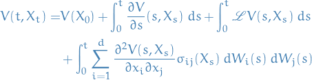
where the generator is defined
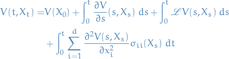
If we further assume that noise in different components are independent, i.e.

then  simplifies to
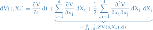
Finally, this can then be written in "differential form":
In pavliotis2014stochastic it is stated that the proof is very similar to the proof of the validity of the proof of the validity of the backward Kolmogorov equation for diffusion processes.
Feynman-Kac formula
- Itô's formula can be used to obtain a probabilistic description of solutions ot more general PDEs of parabolic type
Itô's formula can be used to obtain a probabilistic description of solutions of more general PDEs of parabolic type.
Let be a diffusion process with
- drift
- diffusion

- generator with

and let


be bounded from below.
Then the function
![\begin{equation*}
u(x, t) = \mathbb{E} \bigg[ \exp \bigg( - \int_{0}^{t} V(X_s^x) \ ds \bigg) f(X_t^x) \bigg]
\end{equation*}](../../assets/latex/stochastic_differential_equations_9ecca43052b10d3a9f1ff5b0531aa145d13e6322.png)
is the solution to the IVP
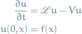
The representation is then called the Feynman-Kac formula of the solution to the IVP.
This is useful for theoretical analysis of IVP for parabolic PDEs of the form above, and for their numerical solution using Monte Carlo approaches.
Examples of solvable SDEs
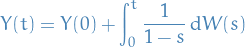
Ornstein-Uhlenbeck process
Properties
- Mean-reverting
- Additive noise
Stuff

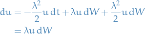
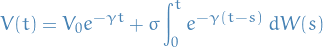
We observe that using Itô's formula
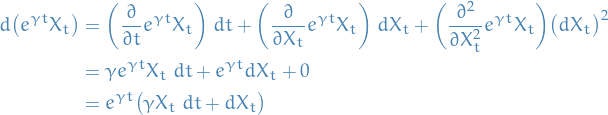
which from the Ornstein-Uhlenbeck equation we see that

i.e.
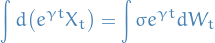
which gives us
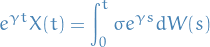
and thus
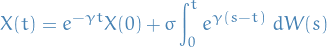
with  assumed to be non-random. This is the solution to the Ornstein-Uhlenbeck process.
Further, we observe the following:
![\begin{equation*}
\mathbb{E} \big[ X(t) \big] = X_0 e^{- \gamma t}
\end{equation*}](../../assets/latex/stochastic_differential_equations_36ffd0487b3958b24eddc2a0dc4a0598723e7152.png)
since this is a Gaussian process. The covariance ew see
![\begin{equation*}
\begin{split}
& \mathbb{E} \big[ \big( X(t) - X_0 e^{- \gamma t} \big) \big( X(s) - X_0 e^{- \gamma t} \big) \big] \\
=\ & \mathbb{E} \bigg[ \bigg( \sigma \int_{0}^{t} e^{\gamma (t' - t)} \ dW(t') \bigg) \bigg( \sigma \int_{0}^{s} e^{\gamma (s' - s)} \ dW(s') \bigg) \bigg] \\
=\ & \sigma^2 \mathbb{E} \bigg[ \bigg( \int_{0}^{s} e^{\gamma (s' - t)} \ dW(s') \bigg) \bigg( \int_{0}^{s} e^{\gamma (s' - s)} \ dW(s') \bigg) \bigg( \int_{s}^{t} e^{\gamma (s' - t)} \ dW(s') \bigg) \bigg] \\
=\ & \sigma^2 \mathbb{E} \bigg[ \bigg( \int_{0}^{s} e^{\gamma (s' - t)} \ dW(s') \bigg) \bigg( \int_{0}^{s} e^{\gamma (s' - s)} \ dW(s') \bigg) \bigg( \int_{s}^{t} e^{\gamma (s' - t)} \ dW(s') \bigg) \bigg]
\end{split}
\end{equation*}](../../assets/latex/stochastic_differential_equations_df6f00842253cdc838d530799f1726b4b9d6bc33.png)
Assuming  , these are independent! Therefore
![\begin{equation*}
\begin{split}
& \mathbb{E} \bigg[ \bigg( \int_{0}^{s} e^{\gamma (s' - t)} \ dW(s') \bigg) \bigg( \int_{0}^{s} e^{\gamma (s' - s)} \ dW(s') \bigg) \bigg( \int_{s}^{t} e^{\gamma (s' - t)} \ dW(s') \bigg) \bigg] \\
= \ & \mathbb{E} \bigg[ \bigg( \int_{0}^{s} e^{\gamma (s' - t)} \ dW(s') \bigg) \bigg( \int_{0}^{s} e^{\gamma (s' - s)} \ dW(s') \bigg) \bigg] \mathbb{E} \bigg[ \bigg( \int_{s}^{t} e^{\gamma (s' - t)} \ dW(s') \bigg) \bigg]
\end{split}
\end{equation*}](../../assets/latex/stochastic_differential_equations_9c7d537e76d7f15bbd3983434c708bbaaa0c4d32.png)
Using Itô isometry, the first factor becomes
![\begin{equation*}
\mathbb{E} \bigg[ \int_{0}^{s} e^{\gamma(2s' - t - s)} \ ds' \bigg] = \frac{1}{2 \gamma} \int_{0}^{s} e^{\tau} \ d \tau = \frac{1}{2 \gamma} \big( e^{s} - 1 \big)
\end{equation*}](../../assets/latex/stochastic_differential_equations_eebe9f22129cc8357346c735d42ae7518bf46662.png)
since
Langevin equation
Notation
- position of particle
 velocity of particle
Definition
Solution
Observe that the Langevin equation looks very similar to the Ornstein-Uhlenbeck process, but with  instead of . We can write this as a system of two SDEs
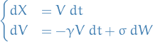
The expression for $d V $ is simply a OU process, and since this does not depend on , we simply integrate as we did for the OU process giving us
Subsituting into our expression for :
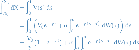
We notice that the integral here is what you call a "triangular" integral; we're integrating from  and integrating
  . We can therefore interchange the order of integration by integrating from
  and the integrating
  from
from  ! In doing so we get:
![\begin{equation*}
\begin{split}
\int_{0}^{t} \int_{0}^{s} e^{- \gamma (s - \tau)} \dd{W(\tau)} \dd{s} &= \int_{0}^{t} \int_{\tau}^{t} e^{- \gamma(s - \tau)} \dd{s} \dd{W(\tau)} \\
&= \int_{0}^{t} - \frac{1}{\gamma} \big( e^{- \gamma (t - \tau)} - 1 \big) \dd{W(\tau)} \\
&= \frac{1}{\gamma} \bigg[ W(t) - \int_{0}^{t} e^{- \gamma (t - \tau)} \dd{W(\tau)} \bigg]
\end{split}
\end{equation*}](../../assets/latex/stochastic_differential_equations_eeff4eee75ee9fa340768570739b462467bd6ef9.png)
Hence the solution is given by

Geometric Brownian motion
The Geometric Brownian motion equation is given by

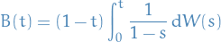
Brownian bridge
Consider the process  which satisfies the SDE
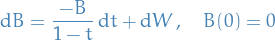
for  .
.
This is the definiting SDE for a Brownian bridge.
Solution

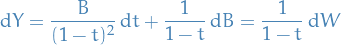
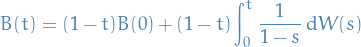
 , we have
A random oscillator
The harmonic oscillator ODE  can be written as a system of ODEs:

A stochastic version might be

where is constant and the frequency is a white noise  with
with  .
.
Solution
We can solve this by letting

so

Then,

Hence,
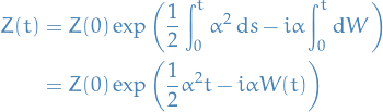
and thus

Stochastic Partial Differential Equations (rigorous)
Overview
This subsection are notes taken mostly from lototsky2017stochastic. This is quite a rigorous book which I find can be quite a useful supplement to the more "applied" descriptions of SDEs you'll find in most places.
I have found some of these more "formal" definitions to be provide insight:
- Brownian motion expressed as a sum over basis-elements multiplied with white noise in each term
- Definition of a "Gaussian process" as it is usually called, instead as a "Guassian field", such that each finite collection of random variables form a Gaussian vector.
Notation

 denotes the space of continuous mappings from metric space
  to metric space
- If
 then we write
- If
 is the collection of functions with
  continuous derivatives
 for
for  and
and  is the collection of functions with continuous derivatives s.t. derivatives of order are Hölder continuous of order
  .
. is the collection of infinitely differentiable functions with compact support
 denotes the Schwartz space and
  denotes the dual space (i.e. space of linear operators on )
 denotes the partial derivatives of every order
 Partial derivatives:
and

- Laplace operator is denoted by

 means
means
and if
 we will write
 means
means

for all sufficiently larger
 .
.
 means that
  is a Gaussian rv. with mean
  and variance
 or
or  are equations driven by Wiener process
- is the sample space (i.e. underlying space of the measure space)
 is the sigma-algebra (
 denotes the power set of )
 is an increasing family of sub-algebras and
  is right-continuous (often called a filtration)
 contains all
  neglible sets, i.e. contains every subset of that is a subset of an element from
  with measure zero (i.e. is complete)
 is an indep. std. Gaussian random variable
Definitions
A filtered probability space is given by
where the sigma-algebra represents the information available up until time .
Let
 be a probability space
 be a filtration
A random process is adapted if is  .
.
This is equivalent to requiring that  for all .
Martingale
A square-integrable Martingale on  is a process
  with values in such that
![\begin{equation*}
M(0) = 0, \quad \mathbb{E} \big[ \left| M(t) \right|^2 \big] < \infty
\end{equation*}](../../assets/latex/stochastic_differential_equations_9ffe6a53f3d1dc8249e53599704599571f3bae44.png)
and
![\begin{equation*}
\mathbb{E} \big[ M(t) \mid \mathcal{F}_s \big] = M(s), \quad \forall t \ge s \ge 0
\end{equation*}](../../assets/latex/stochastic_differential_equations_ebd69bb4c02cbe66f321212917ef7726f74fff4c.png)
A quadratic variation of a martingale  is the continuous non-decreasing real-valued process
  such that

is a martingale.
A stopping (or Markov) time on is a non-negative random variable such that

Introduction
If  is an orthonormal basis in
  , then
is a standard Brownian motion ; a Gaussian process with zero mean and covariance given by
![\begin{equation*}
\mathbb{E} [ w(t) w(s) ] = \min(t, s)
\end{equation*}](../../assets/latex/stochastic_differential_equations_119ad46a2e268146d2f1986e886b86adeea7cdea.png)
This definition of a standard Brownian motion does make a fair bit of sense.
It basically says that that a Brownian motion can be written as a sum of elements in the basis of the space, with each term being multiplied by some white noise.
The derivative of Brownian motion (though does not exist in the usual sense) is then defined
While the series certainly diverges, id oes define a random generalized function on  according to the rule
Consider
- a collection
 of indep. std. Brownian motions,
 orthonormal basis
 in the space
  with
with

a d-dimensional hyper-cube.
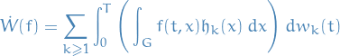
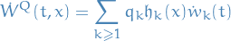
For
 define
Then the process
is Gaussian,
![\begin{equation*}
\mathbb{E}[W(t,x)] = 0, \ \mathbb{E} \big[ W(t, x) W(s, y) \big] = \min(t, s) \prod_{k = 1}^d \min(x_k, y_k)
\end{equation*}](../../assets/latex/stochastic_differential_equations_ad1687b98946456fa75996d1242e479beb3c59ca.png)
We call this process  the Brownian sheet.
From Ex. 1.1.3 b) we have
are i.i.d. std. normal. From this we can define
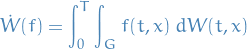
Writing
where  is an orthonormal basis in and
  is an open set.
We call the process  the (Gaussian) space-time white noise. It is a random generalized function
  :
:
Sometimes, an alternative notation is used for  :
:
Unlike the Brownian sheet, space-time white noise is defined on every domain and not just on hyper-cuves  , as log as we can find an orthonormal basis in .
Integrating over 
Often see something like
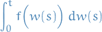
e.g. in Ito's lemma, but what does this even mean?
Consider the integral above, which we then define as
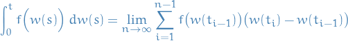
as we would do normally in the case of a Riemann-Stieltjes integral.
Now, observe that in the case of  being Brownian motion, each of these increments are well-defined!
Furthermore, considering a partial sum of the RHS in the above equation, we find that the partial sum converges to the infinite sum in the mean-squared sense.
This then means that the stochastic integral is a random variable, the samples of which depend on the individual realizations of the paths  !
!
Alternative description of Gaussian white noise
Zero-mean Gaussian process
 such that
![\begin{equation*}
\mathbb{E} \big[ \dot{w}(t) \dot{w}(s) \big] = \delta(t - s)
\end{equation*}](../../assets/latex/stochastic_differential_equations_7e27abc40c28cc102d844ee3fb209b275cdd1d69.png)
where
 is the Dirac delta function.
Similarily, we have
![\begin{equation*}
\mathbb{E} \big[ \dot{W}(t, x) \dot{W}(s, y) \big] = \delta(t - s) \delta(x - y)
\end{equation*}](../../assets/latex/stochastic_differential_equations_5e241f6536606487d8e8b936c3e010b756ea9fdb.png)
To construct noise that is white in time and coloured in space, take a sequence of non-negative numbers
 and define
where
is an orthonormal basis in .
We say this noise is finite-dimensional if

Useful Equalities
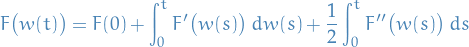
If  is a smooth function and
  is a standard Brownian motion, then
If  is a std. Brownian motion and , an adapted process, then
![\begin{equation*}
\mathbb{E} \Bigg[ \int_{0}^{T} f(t) \ dw(t) \Bigg]^2 = \int_{0}^{T} \mathbb{E} \big[ f^2(t) \big] \ dt
\end{equation*}](../../assets/latex/stochastic_differential_equations_8b5dd42d82b6de2c1f76d33d35465c776e01effe.png)
The Fourier transform is defined
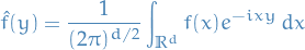
which is defined on the generalized functions from by

for  and
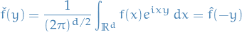
and  . And the inverse Fourier transform is
If is an orthonormal basis in a Hilbert space and  , then
Plancherel's identity (or isometry of the Fourier transform) says that if is a smooth function with compact support in and

then
This result is essentially a continuum version of Parseval's identity.
Useful inequalities
Exercises
1.1.1
![\begin{equation*}
\mathbb{E} [w(t)w(s)] = \min(t,s)
\end{equation*}](../../assets/latex/stochastic_differential_equations_591d6076d829b731d7f3179accb14cfb5bea8d29.png)
Observe that
![\begin{equation*}
w(t) w(s) = \sum_{k}^{} \bigg[ \bigg( \int_{0}^{t} m_k(t') \ dt' \bigg) \xi_k \bigg] \bigg[ \bigg( \int_{0}^{s} m_k(s') \ ds' \bigg) \xi_k \bigg]
\end{equation*}](../../assets/latex/stochastic_differential_equations_c232059185a9dbadd873e9758a41f0411537d0a6.png)
since we're taking the product (see notation). Then, from the hint that  is the Fourier coefficient of the indicator function of the interval
 ![$[0, t]$](../../assets/latex/stochastic_differential_equations_d5bfa804f666bf0df670b0537877972bb84945eb.png) , we make use of the Parseval identity:
, we make use of the Parseval identity:
where  denotes the k-th Fourier coefficient of the indicator function. Then
![\begin{equation*}
\begin{split}
\mathbb{E}[w(t) w(s)] &= \sum_{k}^{} \big( I_t \big)_k \big( I_s \big)_k \mathbb{E}[\xi_k^2] \\
&= \sum_{k}^{} \big( I_t \big)_k \big( I_s \big)_k \\
&= I_t \ I_s \\
&= \min(t, s)
\end{split}
\end{equation*}](../../assets/latex/stochastic_differential_equations_235f44e5fca8101dfc16f9dcb03e03084a27604c.png)
since are all standard normal variables, hence ![$\text{Var}(\xi_k) = \mathbb{E}[\xi_k^2] = 1$](../../assets/latex/stochastic_differential_equations_84e9453ac96933dcaa2e36d51232b5e51a12aa37.png) .
.
I'm not entirely sure about that hint though? Are we not then assuming that the  is the basis? I mean, sure that's fine, but not specified anywhere as far as I can tell?
Hooold, is inner-product same in any given basis? It is! (well, at least for finite bases, which this is not, but aight) Then it doesn't matter which basis we're working in, so we might as well use the basis of  and
and  .
.
1.1.2
Same procedure as in 1.1.1., but observing that we can separate  into a time- and position-dependent part, and again using the fact that
is just the Fourier coefficient of the indicator function on the range ![$[0, x_i]$](../../assets/latex/stochastic_differential_equations_4b4d7b652458d6943b1c96ba194271bbb7937a3a.png) in the i-th dimension.
in the i-th dimension.
Basic Ideas
Notation
- is a probability space
 and
and  are two measurable spaces
 is a random function
- Random process refers to the case when

- Random field corresponds to when
 and .
and .