Numerical Differential Equations
Table of Contents
Notation
 almost always referes to the Lipschitz constant
 refers to LHS of a first-order system
 denotes a "sampled" value of
  at
at  , using our approximation to
  refers to a flow-map, with
  assuming
  (as we can always do)
 refers to the discrete approx. of the flow-map
 refers to the spatial domain, i.e.
  for some
 denote the space of real polynomials of degree
 denotes the i-th abscissa point
Definitions
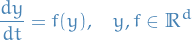
Continuous mechanics
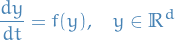
A system of differential equations for which  can be written as a function of
  only is an autonomous-differential-equation (often referred to as continuous mechanics):
Euler's method
We start by taking the Taylor expansion of the solution of the system:
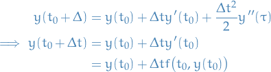
for some ![$\tau \in [t_0, t_0 + \Delta t]$](../../assets/latex/numerical_differential_equations_ae24eff094cbb8854060e5bf67945dc899a4d3e4.png) .
.
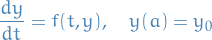
We have the ODE
and the steps are defined as

for

where  denotes our approximation for
  .
.
What we're doing in Euler's method is taking the linear approximation to at each point , but in an interative manner, using our approximation for , at the previous step  to evaluate the point .
This is because we can evaluate  , since
 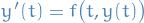 but we of course DON'T know .
y = @(t, y0) (y0 * exp(t) ./ (1 - y0 + y0*exp(t))
y0 = 0.2; T=0:0.5:5; plot(T, y(T, t0));
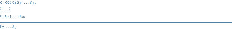
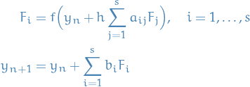
Butcher table

Flow map
Consider the IVP:
which is assumed to have a unique solution on ![$[a, b]$](../../assets/latex/numerical_differential_equations_c9a1e8df376ecb942b106e02d3e6d1b417da2600.png) .
.
The flow map  is then an approximation to a specific solution (a trajectory), i.e. starting at some
  such that
  and
and  , which we write

Observe that it's NOT a discrete approximation, but is continuous.
Adjoint sensitivity analysis
The (local) sensitivity of the solution ot a parameter is defined by how much the solution would change by changes in the parameter, i.e. the sensitivity of the i-th independent variable to the j-th parameter is  .
.
Sensitivity analysis serves two major purposes:
- Diagnostics useful to understand how the solution will change wrt. parameters
- Provides a cheap way to compute the gradient of the solution which can be used in parameter estimation and other optimization tasks
Theorems
Lipschitz convergence
Suppose a given sequence of nonnegative numbers satisfies
where  are nonnegative numbers
  , then, for
Local Existence / Uniqueness of Solutions
Suppose  is:
is:
- continuous
- has continuous partial derivatives wrt. all components of the dependent variable in a neighborhood of the point

Then there is an interval  and unique function which is continuously differentiable on
  s.t. it satisfies
Methods
Euler method
Trapezoidal rule
The Trapezoidal rule computes the average change on the interval ![$[t_n, t_{n + 1}]$](../../assets/latex/numerical_differential_equations_b2f5e1b2fca31fe3098567af2832a78ff743a609.png) , allowing more accurate approximation to the integral, and the update rule is defined as follows:
, allowing more accurate approximation to the integral, and the update rule is defined as follows:
![\begin{equation*}
y_{n + 1} = y_n = \frac{h}{2} \Big[ f(t_n, y_n) + f(t_{n + 1}, y_{n + 1}) \Big]
\end{equation*}](../../assets/latex/numerical_differential_equations_86e7fc1fa54c80bb530ae0f1d26b9740eaade151.png)
Heun-2 (implicit approx. to Trapezoidal rule)
The Heun-2 update rule is an implicit approximation to Trapezoidal rule, where we've replaced the explicit computation of the endpoint  which depend on
  , with a function of the current estimate :
![\begin{equation*}
y_{n + 1} = y_n + \frac{h}{2} \Big[ f(t_n, y_n) + f \big(t_n + h, y_n + h f(t_n, y_n) \big) \Big]
\end{equation*}](../../assets/latex/numerical_differential_equations_23e6b5add77d8f8d2c4570510ffdfecea7620a8a.png)
Convergence of one-step methods
Notation
 denotes the stage values, s.t.
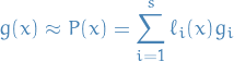
Approximation
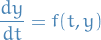
In this chapter we focus on the autonomous differential equation
but the non-autonomous differential equation
can be treated using similar methods.
The global error after  time steps is the difference between the discrete approx. and the exact solution, i.e.

A method is said to be convergent if, for every  ,
,

We have the Taylor expansion given by
for some "perturbation"  about .
For a scalar function, assuming is  times continuously differentiable (i.e.
  ), Taylor's theorem states that
![\begin{equation*}
\exists t^* \in [t, t + \tau] : \quad y(t + \tau) = \sum_{i=0}^{\nu - 1} \frac{\tau^i}{i!} \frac{d^i y}{dt^i}(t) + \frac{\tau^\nu}{\nu!} \frac{d^\nu}{dt^\nu} (t^*)
\end{equation*}](../../assets/latex/numerical_differential_equations_fead1aae8c45680e1420768ad459bcf1a912c05e.png)
Thus, the norm of the last (remainder) term is bounded on ![$[t, t + \tau]$](../../assets/latex/numerical_differential_equations_a78a6ed4d0eb893d00aa7864a018518e735aae50.png) , and we have
, and we have
for some constant  , and thus we write
in general.
For a vector function ( ), Taylor's theorem still holds componentwise, but in general the mean value will be attained at a different
  for each component.
Local error of a numerical method is the difference between the (continuous) flow-map and its (discrete) approx.  :
:

Which measures how much error is introduced in a single timestep of size  .
.
A method is said to be consistent if and only if the local error satisfies
where is a constant that depends on and its derivatives, and  .
.
A method is said to be stable if and only if it satisfies an h-dependent Lipschits condition on (the spatial domain)

where  is not necessarily the Lipschitz constant for the vector field.
Given a differential equation and a generalized one-step method  which is consistent and stable, the global error satisfies
Let the error be

so

Then, adding and subtracting by  ,
,
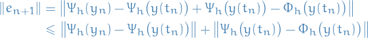
Then, using the fact that the method is consistent and stable, we write
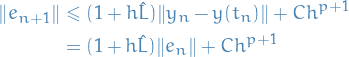
Using this theorem, yields
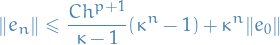
where  . Finally, since
  and therefore
  , if we assume the initial condition is exact (
 ), we get the uniform bound

which proves convergence at order  .
.
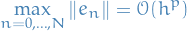
A really good way of estimating the order of convergence for the maximum global error wrt. , is to plot  vs. on a log-log plot since

Thus, is the slope of  .
.
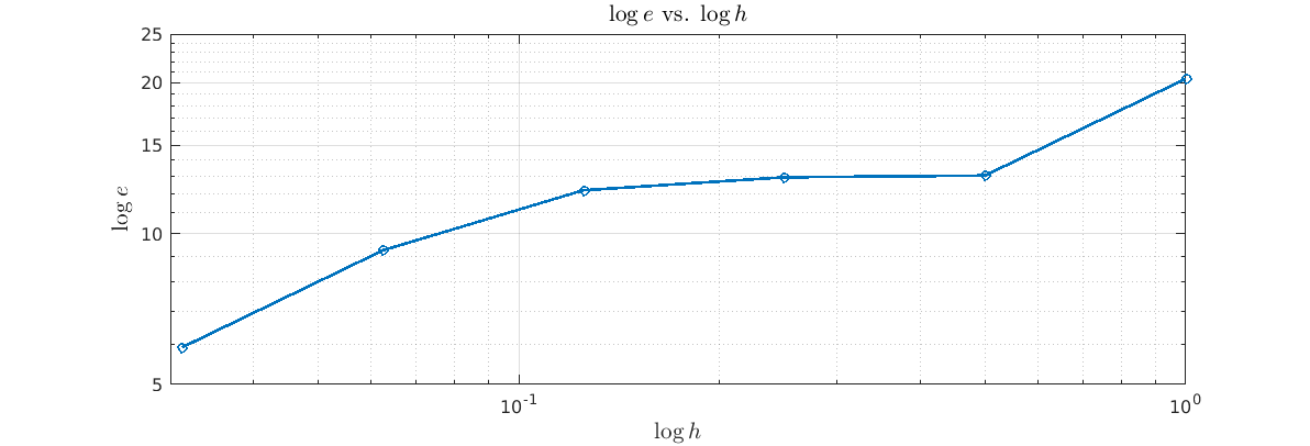
Figure 1: Observe that for smaller values of we have  , i.e. decreases wrt. , while for larger values of we have
  , i.e. decrease in is not even on the order of 1.
Consider a compact domain  and suppose
  is a smooth vector field on and has a Lipschitz constant on (since is smooth, we can take
  ).
).
Then, since
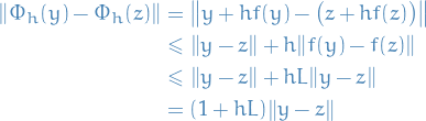
the numerical flow map is Lipschitz with  .
.
The exact solution satisfies
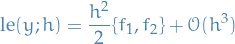
Therefore the local error is
![\begin{equation*}
le(y, h) = y + h f(y) - \Bigg[ y + hf(y) + \frac{h^2}{2} \frac{d^2 y }{dt^2} + \mathcal{O}(h^3) \Bigg] = \mathcal{O}(h^2)
\end{equation*}](../../assets/latex/numerical_differential_equations_3410bed7647f829cf8d930f9adbc7da20d3aefc4.png)
and we can apply the convergence theorem for one-step methods with  to show that Euler's method is convergent with order .
Construction of more general one-step methods
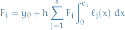
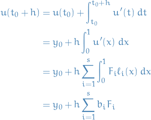
Usually one aims to approximate the integral between two steps:
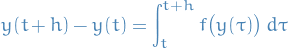
A numerical method to approximate a definite integral of one independent variable is known as numerical quadrature rule.
Example: Trapezoidal rule
The approximation rule becomes:
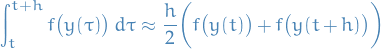
which results in the trapezoidal rule numerical method:

This is an implicit method, since we need to solve for to obtain the step.
Polynomial interpolation
Given a set of abscissa points  and the corresponding data
  , there exists a unique polynomial
  satisfying

called the interpolating polynomial.
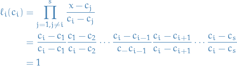
The Lagrange interpolating polynomials  for a set of abscissae are defined by
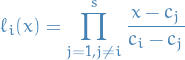
Observe that  then has the property
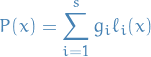
Thus, the set of Lagrange interpolating polynomials form a basis for . In this basis, the interpolating polynomial  assumes the simple form
We also know from Stone-Weierstrass Theorem that the polynomials are dense in  for some compact metric space
  (e.g.
(e.g.  ).
).
Also, if it's not 100% clear why  form a basis, simply observe that if
  then
then
and if  , then we'll multiply by a factor of
  , hence

as wanted. Thus we have  lin. indep. elements, i.e. a basis.
Numerical quadrature
We approximate the definite integral of  based on the interval
 ![$[0, 1]$](../../assets/latex/numerical_differential_equations_68c8fa38d960e53d4308cbf1e65d04c66a554817.png) by exactly integrating the interpolating polynomial of order
by exactly integrating the interpolating polynomial of order  based on
  points
  .
.
The points are known as quadrature points.
We make the following observation:
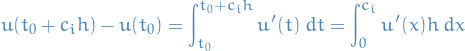
We're interested in approximating the integral of  on the interval
 ![$[t_0, t_0 + h]$](../../assets/latex/numerical_differential_equations_f38efebf139d789519aaac8538255ff29e6b6e1d.png) , thus
, thus
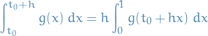
using the change of variables 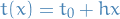 . With the polynomial approx. we then get
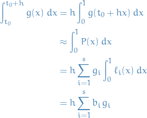
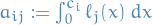
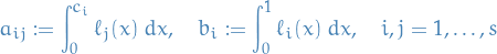
where we've let
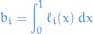
The integral-approximation above is called a quadrature formula.
By construction, a quadrature formula using distinct abscissa points will exactly integrate any polynomial in  (remember that
  are integrals).
We can do better; we say that quadrature rule has order if it exactly integrates any polynomial  . It can be shown that
  always hold, and, for optimal choice of , we have
  .
.
That is, if we want to exactly integrate some polynomial of order , then we only need half as many quadrature points !
import numpy as np
import matplotlib.pyplot as plt
%matplotlib inline
x = np.arange(10)
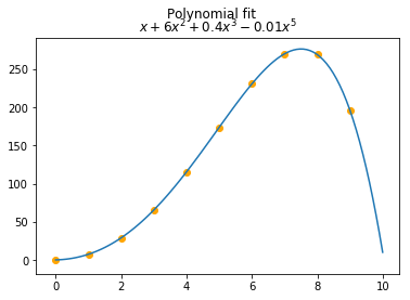
y = x + 6 * x ** 2 + 0.4 * x ** 3 - 0.01 * x ** 5
def polynomial_fit(abscissae, y):
s = abscissae.shape[0]
zeros = np.zeros((s, s - 1))
for i in range(s):
if i == 0:
zeros[i] = x[i + 1:]
elif i == s - 1:
zeros[i] = x[:i]
else:
zeros[i] = np.hstack((x[:i], x[i + 1:]))
denominators = np.prod(abscissae.reshape(-1, 1) - zeros, axis=1) ** (-1)
def p(x):
return np.dot(np.prod(x - zeros, axis=1) * denominators, y)
return p
p = polynomial_fit(x, y)
xs = np.linspace(0, 10, 100)
ys = [p(xs[i]) for i in range(xs.shape[0])]
plt.plot(xs, ys)
plt.suptitle("Polynomial fit")
plt.title("$x + 6x^2 + 0.4x^3 - 0.01x^5$")
_ = plt.scatter(x, y, c="orange")
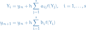
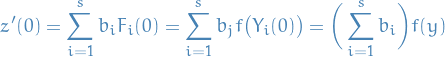
One-step collocation methods
Let  be the collocation polynomial of degree , satisfying
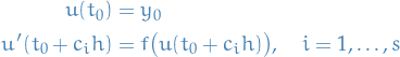
Then we attempt to approximate the gradient as a polynomial, letting  :
:
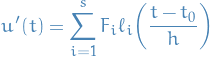
where we've let
Then by the Fundamental Theorem of Calculus, and making the substitution :
And, using our Lagrange polynomial approximation:
we get
Aaand finally,  as stated earlier, hence
for all  . And since
 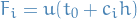 , we get
which gives us a system of (non-linear) equations we need to solve simultaneously.
And therefore, our next step 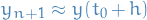 is given by
where we've let
Thus,
Let be the collocation polynomial of degree , satisfying
and let  be the values of the (as of yet undetermined) interpolating polynomial at the nodes:

Then we attempt to approximate the gradient as a polynomial, letting :
The following is something I was not quite getting to grips with, at first.
Now we make the following observation:
by the Fundamental Theorem of Calculus. Thus, making the substitution , gives
And, using our Lagrange polynomial approximation:
we get
Aaand finally, as stated earlier, hence
for all .
Let us denote
Then, a collocation method is given by
where one first solves the coupled sd-dimensional nonlinear system , and the update explicitly.
Important: here we're considering  , rather than the standard , but you can do exactly the same but by plugging in
  in the condition for
  instead of what we just did.
Comparing to interpolating polynomial,  becomes the
  sort of.
Using the collocation methods we obtain a piecewise continuous solution, or rather, a continuous approximation of the solution  on each interval .
In terms of order of accuracy, the optimal choice is attained by using so-called Guass-Legendre collocation methods and placement of nodes at the roots of a shifted Legendre polynomial.
Runge-Kutta Methods
A natural generalization of collocation methods is obtained by:
- allow coefficients ,
 and
and  to take on arbitrary values (not necessarily related to the quadrature rules)
 - no longer assume to be distinct
We then get the class of Runge-Kutta methods!
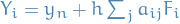
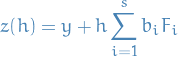
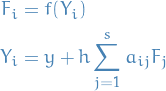
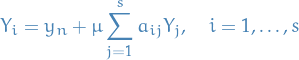
We introduce the stage values  , ending up with what's called the Runge-Kutta methods:
where we can view as the intermediate values of the solution at at time  .
.
For which we use the following terminology:
- the number of stages of the Runge-Kutta method
- are the weights
- are the internal coefficients
Euler's method and trapezoidal rule are Runge-Kutta methods, where

gives us the Euler's method.
If the matrix  is strictly lower-triangular, then the method is explicit.
Otherwise, the method is implicit, as the we might have "circular" dependency between two stages and  , .
, .
Examples of Runge-Kutta methods
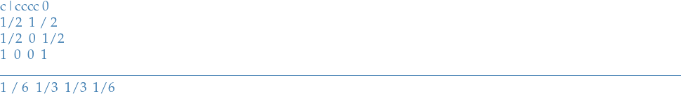
Runge-Kutta method with 4 stages - "THE Runge-Kutta method"
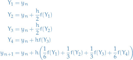
Which often are represented schematically in a Butcher table.
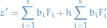
Accuracy of Runge-Kutta methods
Notation
 is the discrete approximation to the flow map, treating as constant
In the case of RK method, we write
where
then
Stuff
- In general, we cannot have an exact expression for the local error

- Can approximate this by computing Taylor expansion wrt.
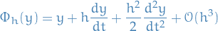
Consider the case of continuous mechanics, the derivates can be related directly to the solution itself by using the differential equation:
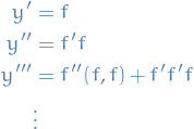
Then, we can write the flow map as
![\begin{equation*}
\Phi_h(y) = y + hf + \frac{h^2}{2} f' f + \frac{h^3}{6} [f''(f, f) + f' ff] + \mathcal{O}(h^4)
\end{equation*}](../../assets/latex/numerical_differential_equations_bf9f7b7fc017af87b37a0cc7ed6b033cfab6dff2.png)
Order conditions for Runge-Kutta methods
With
we have
For the method to have order of , we must have

since we will then have
and thus, the method will be of order . This is the first what is termed as order conditions.
Then, to get the second order condition, we simply compute the second order derivative of  :
:
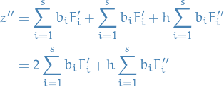
Substituting in the expressions for and , we obtain
Variable stepsize
Notation
 and
and  are two different methods for numerical approximations to the flow map
- is order (local error
 )
) - is order
 (local error
  )
) 
Stuff
Difference in an estimate of the local error by two different methods

And we assume the local error satisfies

i.e. that is the dominating factor.
Error control
Assumptions:
- is a convergent one-step method
- Desire local error at each step less than a given

 estimates the local error at a given point
  when we take a step size of
Idea:
- Estimate the local error with
- If
 then decrease and redo step
 - If
 then keep step; may want to increase
Question: how much do we decrease / increase ?
Suggestion: raise/lower timestep by a factor 
Can be inefficient in the case where we need to do this guessing multiple times, can instead do:
for some
![$\gamma \in [0, 1]$](../../assets/latex/numerical_differential_equations_a22fe950ebf3e28876d24d5ff9e5a489198e88b8.png) , e.g.
, e.g.  , i.e.
  is a decaying factor for the "guess" of the stepsize.
Stability of Runge-Kutta Methods
Notation
 denotes the set of fixed points of the
 denotes the set of fixed points for the numerical estimation of the
  denotes the spectral radius of a matrix
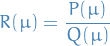
 is the ratio between two polynomials
  and
and  called the stability function
Stuff
An equilibrium point  of the scalar differential equation

is a point for which

Fixed points which are NOT equilibrium points are called extraneous fixed points.
These are points such that

Stability of Equilibrium points
Suppose that in
is  , i.e.
  , and has equilibrium point .
If the eigenvalues of

all lie strictly in the left complex half-plane, then the equilibrium point is asymptotically stable.
If  has any eigenvalue in the right complex half-plane, then is an unstable point.
Stability of Fixed points of maps
We say a numerical method is A-stable if the stability region includes the entire left half-plane, i.e.  is a contained in the stability region.
A A-stable numerical method has the property that it's stable at the origin.
I was wondering why  ? I believe it's because we're looking at solutions which are exponential, i.e.
  , hence if
  , then the exponential will have modulus smaller than 1:

if , for  .
.
We say a numerical method is L-stable if it has the properties:
- it's A-stable
 as
as 
Stability of Numerical Methods
Stability functions
- Scalar case
Consider
 , thus Euler's method has the form
where
Consider the scalar first-order diff. eqn

When applied to this diff. eqn., many methods, including all explicit Runge-Kutta methods, have the form
for some polynomial
.
More generally, all RK methods have the form
where
 is rational polynomial, i.e.
Then we call
 the stability function of the RK method.
 , then we can write this sum in a matrix form:

which has the solution
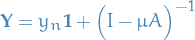
and therefore, finally, we can write


which gives us the stability function
for RK:

Stability of Numerical Methods: Linear case
Linear system of ODEs

where  is diagonalisable. Can write solution as

where  is a diagonalisable matrix.
Further, let an RK method be given with stability function . The origin is stable for numerical method is stable if and only if

Linear Multistep Methods
Notation
 where
where
Definitions
A linear k-step method is defined as
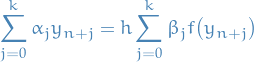
where  and either
  or
or  .
.
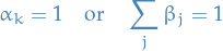
The coefficients are usually normalized such that either
In implementation is's assumed that the values 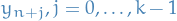 are already computed, so that
  is the only unknown in the formula.
If  is non-zero the method is implicit, otherwise it's explicit.
Examples
 method - generalization of one-step methods
The multistep method is of the form

which is a linear k-step method with coefficients  ,
,  ,
,  and
and  .
.
Examples:
 gives the Forward Euler
 gives the Backwards Euler
 gives the Trapezoidal rule
Leapfrog
 ) given by

 ,
,  and
and  .
.
Adams methods
The class of Adams methods have


 for
for 
If we also have the additional  , we have explicit Adams methods, known as Adams-Bashforth methods, e.g.
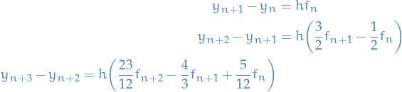
where  .
.
Adams-Moulton methods are implicit, i.e.  .
.
Backward differentiation formulae (BDF)
The Backward differentiation formulae (BDF) are a class of linear multistep methods satisfying
and generalizing backward Euler.
E.g. the two-step method (BDF-2) is
Order of accuracy
Associated with the linear multistep method are the polynomials
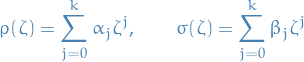
Let be the exact solution at times  for
for  .
.
Then, subsituting into the linear k-step method expression
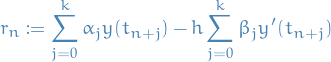
(which is actually the residual accumulated in the  th step, but for notational convenience we will denote it
  ).
).
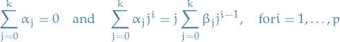
A linear multistep method has order of consistency if (with being the residual)
for all sufficiently smooth , or (it can be shown) equivalently have the following properties:
Coeffiicents
 and
and  satisfy
The polynomials
 and
and  satisfy
The polynomials
and satisfy
Unlike the single-step methods, e.g. Euler method, consistency is insufficient to ensure convergence!
Convergence
A linear multistep method is said to satisfy the root condition, if all roots  of
of

lie in the unit disc, i.e.  , and any root on the boundary, i.e.
  , has algebraic multiplicity one.
Otherwise, the modulus of the solution grows in time.
Suppose a linear multistep method is quipped with a starting procedure satisfying

Then the method converges to the exact solution of
![\begin{equation*}
\frac{dy}{dt} = f(t, y), \quad y(t_0) = y_0, \quad t \in [t_0, t_0 + T]
\end{equation*}](../../assets/latex/numerical_differential_equations_b738a47ef35fe06afe72dacf184c501b2dbee53f.png)
on a fixed interval as  if and only if it has order of accuracy and satisfies the root condition.
Weak Stability and the Strong Root Condition
A convergent multistep method has to be:
- Consistent: so
 and
and  where
where  and
and  are the characteristic polynomials
 Initialized with a convergent starting procedure: i.e. a method to compute
 for the first multistep iteration, to get started, satisfying

- Zero-stable: i.e. it satisfies the root condition; the roots of
 are in the unit disc and simple if on the boundary.
If they're not simple, we get

as we iterate, which is a problem!
We refer to a multistep method that is zero-stable but which has some extraneous roots on the boundary of the unit disk as a weakly stable multistep method.
Same as root condition, but all roots which are not  are within the unit disk.
Asymptotic Stability
The stability region  of a linear multistep method is the set of all points
  such that all roots of the polynomial equation
lie on the unit disc , and those roots with modulues one are simple.
On the boundary of the stability region , precisely one root has modulus one, say  . Therefore an explicit representation for the boundary of is:
![\begin{equation*}
\partial \mathcal{S} = \left\{ z = \frac{\rho(e^{i \theta})}{\sigma(e^{i \theta})} : \theta \in [- \pi, \pi] \right\}
\end{equation*}](../../assets/latex/numerical_differential_equations_109fb547643b88491e8fa60c927989fdf4d39cf0.png)
This comes from applying the multistep method to the diff. eqn. (Dahlquist test equation)
Then
Letting , we get
For any , this is a recurrence relation / linear difference with characteristic polynomial
The stability region is s.t. all roots of  lie in the unit disc and those on the boundary are simply, which is just what we stated above.
Geometric Integration
Focused on constructing methods for specific problems to account for properties of the system, e.g. symmetry.
Notation
First integrals
For some special functions  we may find that is constant along every solution to an /autonomous differential equation
Such a function is called a first integral.
This closely related to the conservation we in Hamiltonian physics.
Let
have a quadratic first integral. A Runge-Kutta method preserves this quadratic first integral if
Splitting methods
- Useful for constructing methods with specific properties
Suppose we wish to solve the differential equation
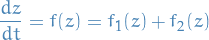
where each of the two differential equations
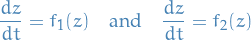
happen to be completely integrable (i.e. analytically solvable).
Then, any point in the phase space, the vector field can be written as two compontents  and
and  . We first step forward along one tangent, and then step forward in the second, each time for a small timestep .
That is, we start from some point  and solve first the IVP
for time , which takes us to the point  where
where  represents the exact solution of the differential equations on vector field .
Next, we start from  and solve the IVP
for time , taking us to the point  .
.
Denoting the flow maps of the vector fields and as  and
and  we have just computed

Such a method is called a splitting method.
The splitting method  where
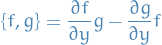
where  , has local error
where  are the commutator of the vector fields and , which is another vector field
More generally
The splitting method where , has local error

where are the commutator of the vector fields and , which is another vector field
If the fields commute, i.e.  , then the splitting is exact.