Analysis
Table of Contents
Defintions
General
The support of a real-valued function  is given by

Lp space
 spaces are function spaces defined using a generalization of the p-norm for a finite-dimensional vector space.
p-norm
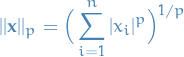
Let  be a real number. Then p-norm (also called the
  -norm) of vectors
  , i.e. over a finite-dimensional vector space, is
Banach space
A Banach space is a vector space with a metric that:
- Allows computation of vector length and distance between vectors (due to the metric imposed)
- Is complete in the sense that a Cauchy sequence of vectors always converge to a well-defined limit that is within the space
Sequences
Sequences of real numbers
Definition of a convergent sequence

 such that
 such that
Bounded sequences
A bounded sequence  such that
Cauchy Sequence
A sequence of points  is said to be Cauchy (in
  ) if and only if for every
  there is an
  such that

For a real sequence this is equivalent of convergence.
TODO Uniform convergence
Series of functions
Pointwise convergence
Let  be a nonempty subset of . A sequence of functions
  is said to converge pointwise on if and only if
  exists for each
  .
.
We use the following notation to express pointwise convergence :

Remarks
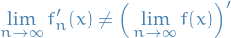
- The pointwise limit of continuous (respectively, differentiable) functions is not necessarily continuous (respectively, differentiable).
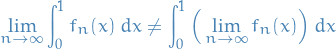
- The pointwise limit of integrable functions is not necessarily integrable.
- There exist differentiable functions
 and
and  such that
  pointwise on $[0, 1], but
- There exist continuous functions and such that pointwise on $[0, 1] but
Uniform convergence
Let be a nonempty subset of . A sequence of functions is said to converge uniformly on to a function if and only if for every  .
.
Continuity
Lipschitz continuity
Given two metric spaces  and
and  , where
  denotes the metric on
  , and same for
  and
and  , a function
  is called Lipschitz continuous if there exists a real constant
  such that

Where the constant  is referred to as the Lipschitz constant for the function .
If the Lipschitz constant equals one,  , we say is a short-map.
If the Lipschitz constant is

we call the map a contraction or contraction mapping.
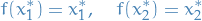
A fixed point (or invariant point )  of a function is an element of the function's domain which is mapped onto itself, i.e.

Observe that if a function crosses the line  , then it does indeed have a fixed point.
The mean-value theorem can be incredibly useful for checking if a mapping is a contraction mapping, since it states that

for some  .
.
Therefore, if there exists  such that
  for all
  then we clearly know that
hence it's a contraction.
Hölder continuity
A real- or complex-valued function on a d-dimensional Euclidean space is said to satisfy a Hölder condition or is Hölder continuous if there exists non-negative  and
and  such that

for all  in the domain of .
This definition can easily be generalized to mappings between two different metric spaces.
Observe that if  , we have Lipschitz continuity.
Càdlàg function
Let  be a metric space, and let
  .
.
A function  is called a càdlàg function if, for very
  :
:
The left limit
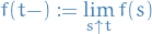
exists.
The right limit
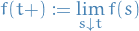
exists and equals

That is, is right-continuous with left limits.
Affine space
An affine space generalizes the properties of Euclidean spaces in such a way that these are independent of concepts of distance and measure of angles, keeping only properties related to parallelism and ratio of lengths for parallel line segments.
In an affine space, there is no distinguished point that serves as an origin. Hence, no vector has a fixed origin and no vector can be uniquely associated to a point. We instead work with displacement vectors, also called translation vectors or simply translations, between two points of the space.
More formally, it's a set  to which is associated a vector space
  and a transistive and free action
  of the additive group of . Explicitly, the definition above means that there is a map, generally denoted as an addition

which has the following properties:
- Right identity: $∀ a ∈ A, a + 0 = 0 $
Associativity:

- Free and transistive action: for every
 , the restriction of the group action to
 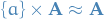 , the induced mapping
  is a bijection.
 - Existence of one-to-one translations: For all
 , the restriction of the group action to
 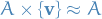 , the induced mapping
  is a bijection.
This very rigorous definition might seem very confusing, especially I remember finding

to be quite confusing.
"How can you map from some set to itself when clearly the LHS contains an element from the vector space !?"
I think it all becomes apparent by considering the following example:  and
and  . Then, the map

Simply means that we're using the structure of the vector space  to map an element from
  to !
to !
Could have written
to make it a bit more apparent (but of course, a set does not have any inherit struct, e.g. addition).
Schwartz space
The Schwartz space  is the space of all
  functions
  on s.t.
for all  .
.
Here if  then
then  and
and
An element of the Schwartz space is called a Schwartz function.
Covering and packing
Let
 be a normed space
We say a set of points  is an
is an  of if
of if
or, equivalently,
The packing number of  as
as

Theorems
Cauchy's Theorem
This theorem gives us another way of telling if a sequence of real numbers is Cauchy.
Let  be a sequence of real numbers. Then is Cauchy if and only if
converges (to some point
be a sequence of real numbers. Then is Cauchy if and only if
converges (to some point  in
in  ).
).
Suppose that is Cauchy. Given  , choose such that

By the Triangle Inequality,

Therefore, is bounded by  .
.
By the Bolzano-Weierstrass Theorem
Telescoping series
Bolzano-Weierstrass Theorem
A sequence  of sets is said to be nested if

If is a nested subsequence of nonempty bounded intervals, then
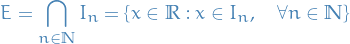
is non-empty (i.e. contains at least one number).
Moreover, if  then contains exactly one number (by non-emptiness of ).
Each bounded sequence in has a convergent subsequence.
Assume that is the lower and  the upper bound of the given sequence. Let
 ![$I_0 = [a, b]$](../../assets/latex/analysis_16e730a333aaf5ac1faa3b4cef202874f95554ac.png) .
.
Divide  into two halves,
  and
and  :
:
![\begin{equation*}
I' = \Bigg[a, \frac{a + b}{2} \Bigg], \quad I'' = \Bigg[ \frac{a + b}{2}, b \Bigg]
\end{equation*}](../../assets/latex/analysis_285aef4cb0f4dc7ec2c3fd6fb02cc01eb8f95f0c.png)
Since  at least one of these intervals contain
  for infinitively many values of
  . We denote the interval with this property
  . Let
. Let  be such that
  .
.
We proceed by induction. Divide the interval  into two halves (like we did with ). At least one of the two halves will contain infinitively many , which we denote
  . We choose
  such that
  .
.
Observe that  is a nested subsequence of boudned and closed intervals, hence there exists
  that belongs to every interval
  .
.
By the Squeeze Theorem  as
as  .
.
Triangle Inequality

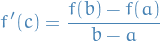
Mean Value Theorem
If a function is continuous on the closed interval ![$[a, b]$](../../assets/latex/analysis_c9a1e8df376ecb942b106e02d3e6d1b417da2600.png) , and differentiable on the open interval
, and differentiable on the open interval  , then there exists a point in such that:
Rolle's Theorem
Suppose  with
with  . If is continuous on , differentiable on and
  then
then  for some
  .
.
Intermediate Value Theorem
Consider an interval ![$I = [a, b]$](../../assets/latex/analysis_f5678fa616e44d479ff19a74dbf6956a9abbbf8c.png) on and a continuous function
on and a continuous function  . If
. If  is a number between
  and
and  , then


M-test
Let be a nonempty subset of and
and suppose
(i.e. series is bounded ).
If  for , then

converges absolutely and uniformly on .
Fixed Point Theory
Banach Fixed Point Theorem
Let  be a be non-empty complete metric space with a contraction mapping
  . Then admits a unique fixed-point in .
Furthermore, can be found as follows:
Start with an arbitrary element  in and define a sequence by
  , then
When using this theorem in practice, apparently the most difficult part is to define the domain such that  .
.
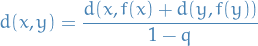
Fundamental Contraction Inequality
By the triangle inequality we have
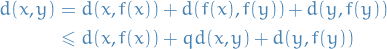
Where we're just using the fact that for any two different  and
and  ,
,  is at least less than
  by assumption of being a contraction mapping.
Solving for  we get
Measure
Definition
A measure on a set is a systematic way of defining a number to each subset of that set, intuitively interpreted as size.
In this sense, a measure is a generalization of the concepts of length, area, volume, etc.
Motivation
The motivation behind defining such a thing is related to the Banach-Tarski paradox, which says that it is possible to decompose the 3-dimensional solid unit ball into finitely many pieces and, using only rotations and translations, reassemble the pieces into two solid balls each with the same volume as the original. The pieces in the decomposition, constructed using the axiom of choice, are non-measurable sets.
Informally, the axiom of choice, says that given a collecions of bins, each containing at least one object, it's possible to make a selection of exactly one object from each bin.
Measure space
If is a set with the sigma-algebra  and the measure
  , then we have a measure space .
Sigma-algebra
Let be some set, and let  be its power set. Then the subset
  is a called a σ-algebra on if it satisfies the following three properties:

- is closed under complement: if
- is closed under countable unions: if

These properties also imply the following:

- is closed under countable intersections: if

A measure on a measure space  is said to be sigma-finite if can be written as a countable union of measurable sets of finite measure.
Borel sigma-algebra
Any set in a topological space that can be formed from the open sets through the operations of:
- countable union
- countable intersection
- complement
is called a Borel set.
Thus, for some topological space , the collection of all Borel sets on forms a σ-algebra, called the Borel algebra or Borel σ-algebra .
Borel sets are important in measure theory, since any measure defined on the open sets of a space, or on the closed sets of a space, must also be defined on all Borel sets of that space. Any measure defined on the Borel sets is called a Borel measure.
Lebesgue sigma-algebra
Basically the same as the Borel sigma-algebra but the Lebesgue sigma-algebra forms a complete measure.
- Note to self
Suppose we have a Lebesgue mesaure on the real line, with measure space
 .
.
Suppose that
is non-measurable subset of the real line, such as the Vitali set. Then the  measure of
  is not defined, but
and this larger set (
 ) does have measure zero, i.e. it's not complete !
- Motivation
Suppose we have constructed Lebesgue measure on the real line: denote this measure space by
. We now wish to construct some two-dimensional Lebesgue measure on the plane  as a product measure.
Naïvely, we could take the sigma-algebra on
to be  , the smallest sigma-algebra containing all measureable "rectangles"
  for
for  .
.
While this approach does define a measure space, it has a flaw: since every singleton set has one-dimensional Lebesgue measure zero,

for any subset of
.
What follows is the important part!
However, suppose that
is non-measureable subset of the real line, such as the Vitali set. Then the measure of is not defined (since we just supposed that is non-measurable), but
and this larger set (
) does have measure zero, i.e. it's not complete !
- Construction
Given a (possible incomplete) measure space
 , there is an extension
  of this measure space that is complete .
The smallest such extension (i.e. the smallest sigma-algebra
 ) is called the completion of the measure space.
It can be constructed as follows:
- Let
 be the set of all measure zero subsets of (intuitively, those elements of that are not already in are the ones preventing completeness from holding true)
 - Let be the sigma-algebra generated by and (i.e. the smallest sigma-algreba that contains every element of and of )
- has an extension to (which is unique if is sigma-finite), called the outer measure of , given by the infimum

Then
is a complete measure space, and is the completion of .
What we're saying here is:
- For the "multi-dimensional" case we need to take into account the zero-elements in the resulting sigma-algebra due the product between the 1D zero-element and some element NOT in our original sigma-algebra
- The above point means that we do NOT necessarily get completeness, despite the sigma-algebras defined on the sets individually prior to taking the Cartesian product being complete
- To "fix" this, we construct a outer measure
 on the sigma-algebra where we have included all those zero-elements which are "missed" by the naïve approach,
- Let
Product measure
Given two measurable spaces and measures on them, one can obtain a product measurable space and a product measure on that space.
A product measure  is defined to be a measure on the measurable space
  , where we've let
  be the algebra on the Cartesian product
  . This sigma-algebra is called the tensor-product sigma-algebra on the product space.
A product measure is defined to be a measure on the measurable space satisfying the property

Complete measure
A complete measure (or, more precisely, a complete measure space ) is a measure space in which every subset of every null set is measurable (having measure zero).
More formally, is complete if and only if

Lebesgue measure
Given a subset , with the length of a closed interval ![$I = [a,b]$](../../assets/latex/analysis_3fdf3f4bf882725c6261a1b413e5bc0b103e1281.png) given by
given by  , the Lebesgue outer measure
  is defined as

The Lebesgue measure is then defined on the Lebesgue sigma-algebra, which is the collection of all the sets which satisfy the condition that, for every 

For any set in the Lebesgue sigma-algrebra, its Lebesgue measure is given by its Lebesgue outer measure  .
.
IMPORTANT!!! This is not necessarily related to the Lebesgue integral! It CAN be be, but the integral is more general than JUST over some Lesgue measure.
Intuition
- First part of definition states that the subset is reduced to its outer measure by coverage by sets of closed intervals
- Each set of intervals
 covers in the sense that when the intervals are combined together by union, they contain
 - Total length of any covering interval set can easily overestimate the measure of , because is a subset of the union of the intervals, and so the intervals include points which are not in
Lebesgue outer measure emerges as the greatest lower bound (infimum) of the lengths from among all possible such sets. Intuitively, it is the total length of those interval sets which fit most tightly and do not overlap.
In my own words: Lebesgue outer measure is smallest sum of the lengths of subintervals s.t. the union of these subintervals completely "covers" (i.e. are equivalent to) .
If you take an a real interval , then the Lebesge outer measure is simply  .
.
Lebesgue Integral
The Lebesgue integral of a function over a measure space is written

which means we're taking the integral wrt. the measure .

Special case: non-negative real-valued function
Suppose that  is a non-negative real-valued function.
Using the "partitioning of range of " philosophy, the integral of should be the sum over  of the elementary area contained in the thin horizontal strip between
  and
and  , which is just
Letting

The Lebesgue integral of is then defined by
where the integral on the right is an ordinary improper Riemann integral. For the set of measurable functions, this defines the Lebesgue integral.
Measurable function
Let  and
and  be measurable spaces.
A function  is said to be measurable if the preimage of under is in for every
  , i.e.

Radon measure
- Hard to find a good notion of measure on a topological space that is compatible with the topology in some sense
- One way is to define a measure on the Borel set of the topological space
Let be a measure on the sigma-algebra of Borel sets of a Hausdorff topological space .
- is called inner regular or tight if, for any Borel set
 ,
,  is the supremum of
  over all compact subsets of of
 - is called outer regular if, for any Borel set , is the infimum of
 over all open sets
  containing
 - is called locally finite if every point of has a neighborhood for which is finite (if is locally finite, then it follows that is finite on compact sets)
The measure is called a Radon measure if it is inner regular and locally finite.
Suppose and  are two
  measures on a measures space
  and that is absolutely continuous wrt. .
Then there exists a non-negative, measurable function  on such that
The function is called the density or Radon-Nikodym derivative of wrt. .
Continuity of measure
Suppose and are two sigma-finite measures on a measure space  .
.
Then we say that is absolutely continuous wrt. if

We say that and are equivalent if each measure is absolutely continuous wrt. to the other.
Density
Suppose and are two sigma-finite measures on a measure space and that is absolutely continuous wrt. . Then there exists a non-negative, measurable function on such that
Measure-preserving transformation
 is a measure-preserving transformation is a transformation on the measure-space if
Sobolev space
Notation
 is an open subset of
  denotes a infinitively differentiable function
  with compact support
- is a multi-index of order
 , i.e.
Definition
Vector space of functions equipped with a norm that is a combination of norms of the function itself and its derivatives to a given order.
Intuitively, a Sobolev space is a space of functions with sufficiently many derivatives for some application domain, e.g. PDEs, and equipped with a norm that measures both size and regularity of a function.
The Sobolev space spaces  combine the concepts of weak differentiability and Lebesgue norms (i.e. spaces).
For a proper definition for different cases of dimension of the space  , have a look at Wikipedia.
Motivation
Integration by parst yields that for every  where
where  , and for all infinitively differentiable functions with compact support :
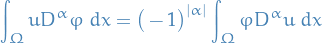
Observe that LHS only makes sense if we assume to be locally integrable. If there exists a locally integrable function  , such that
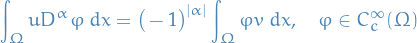
we call the weak -th partial derivative of . If this exists, then it is uniquely defined almost everywhere, and thus it is uniquely determined as an element of a Lebesgue space (i.e. function space).
On the other hand, if , then the classical and the weak derivative coincide!
Thus, if  , we may denote it by
  .
.
Example
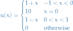
is not continuous at zero, and not differentiable at −1, 0, or 1. Yet the function
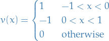
satisfies the definition of being the weak derivative of  , which then qualifies as being in the Sobolev space
  (for any allowed
  ).
).
Ergodic Theory
Let be a measure-preserving transformation on a measure space with  , i.e. it's a probability space.
Then  is ergodic if for every
  we have

Limits of sequences
Infinite Series of Real Numbers
Theorems
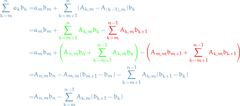
Abel's formula
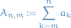
Let  and
and  be real sequences, and for each pair of integers
  set
set
Then
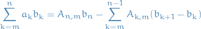
for all integeres  .
.
Since 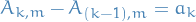 for
for  and
and  , we have
Infinite Series of Functions
Uniform Convergence
Theorems
Cauchy criterion
Let be a nonempty subset of , and let be a sequence of functions.
Then converges uniformly on if and only if for every there is an  such that

for all .
Generally about uniform convergence
Let be a nonempty subset of and let  be a sequence of real functions defined on
i) Suppose that  and that each
  is continuous at . If
  converges uniformly on , then is continuous at
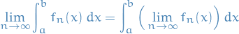
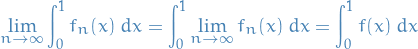
ii) [Term-by-term integration] Suppose that ![$E = [a, b]$](../../assets/latex/analysis_b2cd9898000992bba39f8c5b726ba5372034ca64.png) and that each is integrable on . If converges uniformly on , then is integrable on and
and that each is integrable on . If converges uniformly on , then is integrable on and
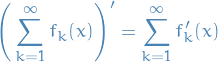
iii) [Term-by-term differentiation] Suppose that is a bounded, open interval and that each is differentiable on . If  converges at some , and
  converges uniformly on , then
  converges uniformly on , is differentiable on , and
Suppose that uniformly on a closed interval . If each is integrable on , then so is and
In fact,
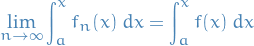
uniformly on ![$x \in [a, b]$](../../assets/latex/analysis_2d517a1540844b320724f283341b89b5a9c92577.png) .
.
Problems
7.2.4
Let
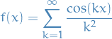
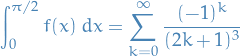
- Show that the series converges on
![$[0, \frac{\pi}{2}]$](../../assets/latex/analysis_2ab3b0e0ae3632b24a23b25b4ec68039f3ab2cad.png)
- We can integrate series term by term
Start by bounding the terms in the sum:
And since the series  converges, the series in question converges.
Further,
![\begin{equation*}
\begin{align}
\int_0^{\pi / 2} f(x) dx &= \sum_{k=1}^\infty \int_0^{\pi / 2} \frac{\cos kx}{k^2} \ dx \\
&= \sum_{k=1}^\infty \Big[ \frac{\sin kx}{k^3} \Big]_0^{\pi / 2} \\
&= \sum_{k=1}^\infty \frac{\sin (k \pi / 2)}{k^3}
\end{align}
\end{equation*}](../../assets/latex/analysis_0e8acf3f08bd65d77e0a4a7b036002bf65bb6c6c.png)
Here we note that the numerator will only take on the values  , and in the non-zero cases the denominator will be as in the claim.
TODO 7.2.5
converges pointwise on and uniformly on each bounded interval in to a differentiable function which satisfies

for all
- Pointwise convergence on
- Uniform convergence with
For 1. we observe that
![\begin{equation*}
\mathbb{R} = \underset{m \ge 1}{\cup} [ -m, m]
\end{equation*}](../../assets/latex/analysis_6f5476a8bdb9d58f0ea2313913f8e88aaaaa6263.png)
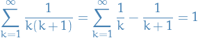
where the last step is due to the sum being a Telescoping series, which equals 1.
We then use the M-test, hence we get convergence in uniform on .
Now that we know that the series converges, we need to establish that the function satisfies the boundaries.
Where  becomes
  if we can prove that RHS converges.
TODO 7.2.6
- Look at the more general case
- Look also at

Workshop 2
- 6
- Question
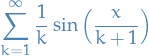
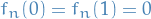
Let
 for
for ![$x \in [0, 1]$](../../assets/latex/analysis_1abcf6a6ba0996351c652ec55b2a137f25774cfc.png) . Prove that converges pointwise on
. Prove that converges pointwise on ![$[0, 1]$](../../assets/latex/analysis_68c8fa38d960e53d4308cbf1e65d04c66a554817.png) and find the limit function.
Is the convergence uniform on ? Is the convergence uniform on
and find the limit function.
Is the convergence uniform on ? Is the convergence uniform on ![$[a, 1]$](../../assets/latex/analysis_cb441010393ff7a0abf0e50800c1ad385443f0ba.png) with
with  ?
?
- Answer
First observe that for
 and
and  we have
And for


Therefore the limiting function is

Is the convergence uniform on
? No!
By Thm. 7.10 in introduction_to_analysis we know that if uniformly then
but in this case
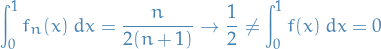
Hence we have a proof by contradiction.
Is the convergence uniform on
? Yes!

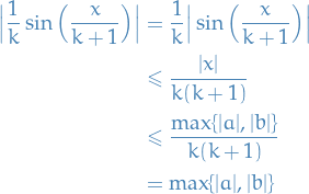
and

hence
uniformly on for .
- Question
- 7
- Question
Let
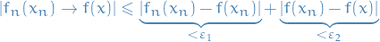
 be a sequence of continuous functions which converge uniformly to a function
  . Let
. Let  be a sequence of real numbers which converges to . Show that
 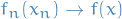 .
.
- Answer
Observe that
for some
 and
and  . We know

and for all


Further, by Theorem 7.10 introduction_to_analysis,

which implies

Therefore, for
, let

and
then

as wanted.
- Question
Uniform Continuity
Theorems
Suppose ![$f: [a, b] \to \mathbb{R}$](../../assets/latex/analysis_ad16c0aff3aa355602aa32a69863fed8f987a882.png) is continuous. Then it is uniformly continuous.
is continuous. Then it is uniformly continuous.
Problems
Workshop 3
- 5
- Question
Let
be an open interval in . Suppose  is differentiable and its derivative
  is bounded on . Prove that is uniformly continuous on .
- Answer
Suppose
for
 . Then by Mean Value theorem we have

Therefore,
Thus, let

Then

Hence
is uniformly continuous.
- Question
Power series
Definitions
Let  be a sequence of real numbers, and
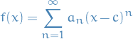
  . A power series is a series of the form
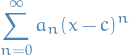
The numbers  are called coefficients and the constant is called the center.
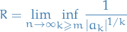
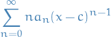
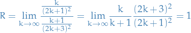
Suppose we have the power series
then the radius of convergence  is given by

unless  is bounded for all
  , in which case we declare
I.e. is the smallest number such that all series with  is bounded.
Analytic functions
We say a function is analytic if it can be expressed as a power-series .
More precisely, is analytic on  if there is a power series which converges to on .
Theorems
This holds in general , thus is basically another way of defining the radius of convergence .
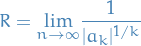
provided this limit exists.
Converges to a continous function
Assume that  . Suppose that
  . Then the power series converges uniformly and absolutely on
  to a continuous function . That is,
Taylor's Theorem
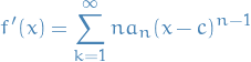
Suppose the radius of convergence is . Then the function
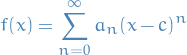
is infinitely differentiable on  , and for such x,
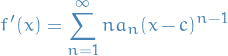
and the series converges absolutely, and also uniformly on ![$[r - c, r + c]$](../../assets/latex/analysis_153f574aa8dc8898ab42019326f68c167645a08d.png) for any $ r < R$. Moreover
for any $ r < R$. Moreover
Consider the series
which has radius of convergence and so converges uniformly on for any  .
.
Since
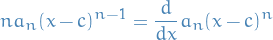
and  at least converges at one point, then by Theorem 7.14 in Wade's we know that
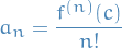
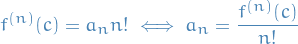
Further, we have  and
and  , which we can keep on doing and end up with
Problems
Finding radius of convergence
The power series

has a radius of convergence  , and converges absolutely on the interval
  .
.
One can easily see that the series convergences on the the interval  , and so we consider the endpoints of this interval.
 convergences
 , which is known as the harmonic series and is known to diverge
7.3.1
a)
The series
converges on the interval , and has radius of convergence .
Letting  we write

Using the Ratio test, gives us
Thus we have the endpoints  and
and  .
.
For we get the series
which converges.
For  we get the series
for which we can use the alternating series test to show that it converges.
Thus, we have the series converging on the interval .
b)
We observe that
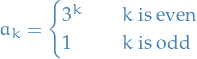
and let  , writing the series as

and using the root test, we get
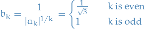
where we let the above equal  for the sake of convenience.
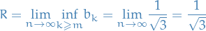
Then we use the lim-inf definition of radius of convergence
c)

7.3.2
a)
Look at solution to 7.3.1. a)
b)
c)
Integrability on R
Definitions
Partition
Let with
i) A partition of the interval ![$[a,b]$](../../assets/latex/analysis_bf64a90d032efdc91fa5aab3916a535ed7759bfd.png) is a set of points
is a set of points  such that

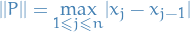
ii) The norm of a partition 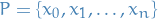 is the number
iii) A refinement of a partition is a partition  of which satisfies
  . In this case we say that is finer than
  .
.
Riemann sum
Let with , let 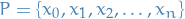 be a partition of the interval , set
  for
for  and suppose that
 ![$f : [a, b] \to \mathbb{R}$](../../assets/latex/analysis_7ae547159e883a60c88d3c5ad37403c18e8f1e01.png) is bounded.
is bounded.
i) The upper Riemann/Darboux sum of over is the number
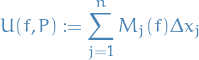
where
![\begin{equation*}
M_j(f) := \sup f([x_{j-1}, x_j]) := \underset{t \in [x_{j-1}, x_j]}{\sup} f
\end{equation*}](../../assets/latex/analysis_a72eb6f326a231e085d67916ecec318f7befc1ec.png)
ii) The lower Riemann/Darboux sum of over is the number
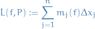
where
![\begin{equation*}
m_j(f) := \inf f([x_{j-1}, x_j]) := \underset{t \in [x_{j-1}, x_j]}{\inf} f
\end{equation*}](../../assets/latex/analysis_87c1f17848cd3a70860929b3794100e042510f95.png)
Since we assumed to be bounded, the numbers  and
and  exist and are finite.
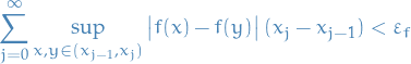
Riemann integrable
Let with . A function is said to be Riemann integrable on if and only if is bounded on , and for every
![\begin{equation*}
\exists P = \{ x_0, x_1, \dots, x_n \} \text{ of } [a, b] \implies U(f, P) - L(f, P) < \varepsilon
\end{equation*}](../../assets/latex/analysis_9a7a40f41811be0c7486f2ca8192d6274395a41c.png)
I.e. the upper and lower Riemann / Darboux sums has to converge to the same value.
Riemann integral
Let with , and be bounded.
i) The upper integral of on is the number
![\begin{equation*}
(U) \int_a^b f(x) \ dx := \inf \Big\{ U(f, P) : P \text{ is a partition of } [a,b] \Big\}
\end{equation*}](../../assets/latex/analysis_9ca9f18de6839e93d2f409f7705f20e06356e4ab.png)
ii) The lower integral of on is the number
![\begin{equation*}
(L) \int_a^b f(x) \ dx := \sup \Big\{ L(f, P) : P \text{ is a partition of } [a,b] \Big\}
\end{equation*}](../../assets/latex/analysis_f0eb8f312a92f72970d221f0d051499b877009c0.png)
iii) If the upper and lower integral are equal, we define the integral to be this number
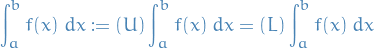
The following definition of the Riemann sum can be proven to be equivalent of the upper and lower integrals using introduction_to_analysis.
Let
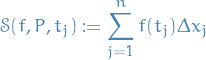
i) A Riemann sum of wrt. a partition  of generated by samples
 ![$t_j \in [x_{j - 1}, x_j]$](../../assets/latex/analysis_4978dc4bc85c39e47478ad104789549be52dc5f5.png) is a sum
is a sum
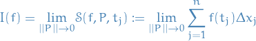
ii) The Riemann sums of are said to converge to  as
as  if and only if given there is a partition
  of
of ![$[a ,b]$](../../assets/latex/analysis_565d83a42343e19c30eb852a9ff2cada768b98cb.png) such that
such that

for all choices of ![$t_j \in [x_{j-1}, x_j], j = 1, 2, \dots, n$](../../assets/latex/analysis_a630f0dbcaa3a7c9e0784f856adce66fc9b14c65.png) . In this case we shall use the notation
. In this case we shall use the notation
 1
1
 is just some arbitrary number in the given interval, e.g. one could set
  .
.
Theorems
Suppose with . If is continuous on the interval , then is integrable on .
Telescoping
If  , then
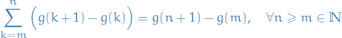
This is more of a remark which is very useful for proofs involving Riemann sums, since we can write
This allows us to write the following inequality for the upper and lower Riemann / Darbaux:

in which case all we need to prove for to be Riemann integrable is that this goes to zero as  , or equiv. as we get a finer partition.
Mean Value Theorem for Integrals
Suppose that and  are integrable on with
  for all . If
![\begin{equation*}
m = \inf f[a, b] \quad \text{and} \quad M = \sup f[a,b]
\end{equation*}](../../assets/latex/analysis_ac26bf0958bb44a3e51160d6c25975bf09116cbc.png)
then
![\begin{equation*}
\exists c \in [a, b] \implies \int_a^b f(x) g(x) \ dx = c \int_a^b g(x) \ dx
\end{equation*}](../../assets/latex/analysis_c5bf5abaf45c5f3d269f0b7cb2da45a15e1cf849.png)
In particular, if is continuous on , then
![\begin{equation*}
\exists x_0 \in [a,b] \implies \int_a^b f(x) g(x) \ dx = f(x_0) \int_a^b g(x) \ dx
\end{equation*}](../../assets/latex/analysis_b4b547dcefe1725421be04d4d582850664ff7aaa.png)
Suppose that  are integrable on , that is nonnegative on , and that
![\begin{equation*}
m, M \in \mathbb{R} : m \le \inf f([a, b]) \text{ and } M \ge \sup f([a, b])
\end{equation*}](../../assets/latex/analysis_db75e06669e29f4e9f7940e72c91354c66632f4a.png)
Then there is an ![$c \in [a, b]$](../../assets/latex/analysis_1b6684a4bf25d39ac19401f8f0498e64c814c7db.png) s.t.
s.t.
In particular, if is also nonnegative on , then there is an which satisifies
Let be a real-valued function which is continuous on the closed interval , must attain its maximum and minimum at least once. That is,
![\begin{equation*}
\exists c, d \in [a, b] : f(c) \le f(x) \le f(d), \quad \forall x \in [a, b]
\end{equation*}](../../assets/latex/analysis_9dd84e773a9b779356517ead54f523ee826c7529.png)
Fundamental Theorem of Calculus
Let be non-degenerate and suppose that .
i) If is continuous on and  , then
 ![$F \in \mathcal{C}^1 [a, b]$](../../assets/latex/analysis_db8015f30250dd42407ec202a9670eabe00ef24b.png) and
and
![\begin{equation*}
\frac{d}{dx} \int_a^x f(t) \ dt := F'(x) = f(x), \quad \forall x \in [a, b]
\end{equation*}](../../assets/latex/analysis_61fe2abdf6951585784bbe7561466d92248e6c1f.png)
ii) If is differentiable on and is integrable on then
![\begin{equation*}
\int_a^x f'(t) \ dt = f(x) - f(a), \quad \forall x \in [a,b]
\end{equation*}](../../assets/latex/analysis_00b1ac6ee7d2a71e25da6bbc96aeeb9586e73f6e.png)
Non-degenerate interval means that  .
.
Integrability on R (alternative)
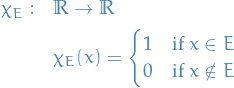
Let . Then we define the characteristic function
Let be a bounded interval, then we define the integral of  as
as
Reminds you about Lebesgue-integral, dunnit?
We say  is a step function if there exist real numbers

such that
 for
for  and
and 
 is constant on
We will use the phrase " is a step function wrt.  " to describe this situation.
In other words, is step function wrt. iff there exists  such that
for  .
.
If is a step function wrt. which takes the value  on
on  , then
Notice that the values  have no effect on the value of
  , as one would expect.
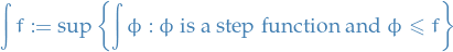
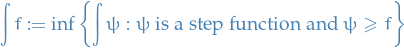
Let . We say that is Riemann integrable if for every there exist step functions and such that

and
A function is Riemann integrable if and only if

 as the common value
A function is Riemann integrable if and only if there exist sequences of step functions  and
and  such that

and
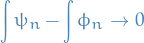
If and are any sequences of step functions satisfying the above, then
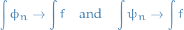
as  .
.
Suppose and are Riemann integrable, and  . Then
 is Riemann-integrable and
If
 then
then  . Further,
 is Riemann integrable and

 and
and  are Riemann integrable
 is Riemann integrable
Integrals and uniform limits of sequences and series of functions
Suppose is a sequence of Riemann integrable functions which

uniformly.
Suppose that and are zero outside some common interval . Then is Riemann integrable and
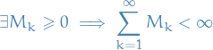
Suppose  is a non-negative sequence of numbers and
  is a function that
For some
and 

For
 we have

Then
for some  .
.
Problems
Workshop 5
5
- Question
- Answer
is Riemann integrable, then there exists step-functions and such that

Or rather, for all
 , there exists
  such that
Since
is integrable on a bounded and closed interval, then is bounded and has bounded support. That is
![\begin{equation*}
\sup_{x \in [a, b]} f(x) \le M
\end{equation*}](../../assets/latex/analysis_6c0719e3cc514f0ab23b33fcc394f47c9ab3a7cd.png)
Therefore, by the Mean Value theorem, we have
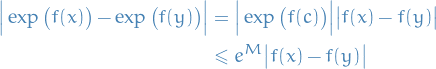
Therefore the "integral sum" for
![$\exp(f) \chi_{[a, b]}$](../../assets/latex/analysis_f4b888411df0037a7c7a441b14f369ad28eab071.png) satisfy the following inequality
satisfy the following inequality

Therefore, for
, we choose

which gives us

That is,
is Riemann integrable implies is Riemann integrable.
We've left out the
![$\chi_{[a, b]}$](../../assets/latex/analysis_bd5a94be38efcaba769bf7a0cc41cb99d3f72501.png) in all the expressions above for brevity, but they ought to be included in a proper treatment.
in all the expressions above for brevity, but they ought to be included in a proper treatment.
 outside of
 ![\begin{equation*}
\big( \exp f \big) \chi_{[a, b]}
\end{equation*}](../../assets/latex/analysis_e375644fca83d837ca4ae811adda2aceb0c8a29f.png)
Metric spaces
Definitions
Metric
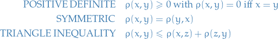
A metric space is a set together with a function  (called the metric of ) which satisfies the following properties for all
  :
:
 2
2
Metric space
A metric space is a set together with a function
(called the metric of ) which satisfies the following properties for all :
3
Balls
Let  and
and  . The open ball (in ) with center and radius
  is the set

Let and . The closed ball (in ) with center and radius is the set

Equivalence of metrics
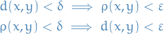
We say two metrics  and on a set are strongly equivalent if and only if

We say two metrics and on a set are equivalent if and only if for every  and every there exists such that
Closedness and openness
 is said to be open if and only if for every
  there is an
  is contained in
  is
is Closure and interior
For 

is the interior of ; it is the largest subset of which is open.
Or equivalently, the interior of a subset of points of a topological space consists of all points of that do not belong to the boundary of .
A point that is in the interior of is an interior point of .
For
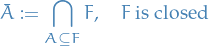
is the closure of ; it is the smallest set containing which is closed .
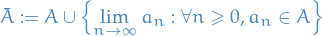
Or, equivalently, the closure of is the union of and all its limit points (points "arbitrarily close to "):
For

is the boundary of .
Convergence, Cauchy sequences and completeness
Most theorems and definitions used for sequences are readily generalized to metric spaces.
We say a metric space is complete if and only if every Cauchy sequence in converges.
In a metric space , a sequence  with
with  is bounded if there exists some ball
  such that
  for all .
In a metric space , a sequence with is a Cauchy sequence iff for every ,

Let be a metric space, then is said to satisfy the Bolzano-Weierstrass Property iff every bounded sequence has a convergent subsequence .
Closedness, limit points, cluster points and completeness
is a limit point for if and only if there is a sequence  such that
  as .
as .
is a cluster point for if and only if every open ball centred at contains infinitely many points of .
The following statements are equivalent:
- s a cluster point for
- for all ,
 contains a point of
  , with
  for all , s.t. as
Every cluster point for is a limit point for . But can be a limit point for without being a cluster point .
A closed subset of a complete metric space is complete
A complete subset of any metric space is closed.
Every convergent sequence is Cauchy, but the opposite is not necessarily true.
Compactness
Let  be a collection of subsets of a metric space and suppose that is a subset of .
 is said to cover if and only if

is said to be an open covering of iff covers and each  is open.
Let be a covering of .
is said to a finite (respectively, countable ) subcovering iff there is a finite (respectively, countable) subset  of s.t.
  covers .
Let be a metric space.
A subset  is compact iff for every open cover
  of , there is a finite subcover
  of .
of .
I often find myself wondering "what's so cool about this compactness?! It shows up everywhere, but why?"
Well, mainly it's just a smallest-denominator of a lot of nice properties we can deduce about a metric space. Also, one could imagine compactness being important since the basis building blocks of Topology is in fact open sets, and so by saying that any open cover has a finite open subcover, we're saying it can be described using "finite topological constructs". But honestly, I'm still not sure about all of this :)
One very interesting theorem which relies on compactness is Stone-Weierstrass theorem, which allows us to show that for example polynomials are dense in the space of continous functions! Suuuuper-important when we want to create an approximating function.
Let  be a metric space and let
  . Then
  is said to be dense in if for every and for every we have that
  i.e., every open ball in contains a point of .
Or, alternatively, as described in thm:dense-iff-closure-eq-superset:

A metric space is said to be separable iff it contains a countable dense subset.
Where with countable dense subset we simply mean a dense subset which is countable.
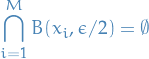
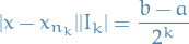
We say the metric space is a precompact metric space if for every there is a cover of by finitely many closed balls of the form

Let be a complete metric space and precompact, then is compact.
Let be a metric space. Then is said to be sequentially compact if and only if every sequence in has a convergent subsequence.
Let be a topological space, and a subspace.
Then is compact (as a topological space with subspace topology) if and only if every cover of by open subsets of has a finite subcover.
If  for
for  open in (subspace topology), then
  open in s.t.
  .
.
Therefore

 : Choose finite subcover
  . Then
  is a finite subcover of .
 : Let
: Let  , then
  open in . So we let
so there exists finite  with
with
Every space with cofinite topology is compact.
Let  . Take some
  so that
  is finite.
Then  , there exists
  in cover with
  . Therefore
is a finite cover.
Idea: take away one cover → left with finitely many points → we good.
Motivation
Let . For which must be bounded?
- finite
- If
 of opens with
  bounded then is bounded.
 Any continuous
is locally bounded

with
 bounded, e.g.
If there exists finitely many
 as above, with

then
is bounded.
Compactness NOT equivalent to:
 is a cover of
  covers but not finite.
 cover → clearly not finite mate
- Same as 2, but take finitely many
- Follows from 2 by taking subcover to be the whole cover.
 always covers and has finite subcover (e.g.
  )
)
Examples
- Non-compact
 , so
, so  has no finite subcover, so not compact
- Infinite discrete space is not compact. Consider
 which is an open cover, but has no finite subcover.
- Compact
- indiscrete so
 . Only open covers are and
  , and is a finite subcover, hence is compact.
 - Any finite space is compact (for any topology)
Some specific spaces
Banach space
See Banach space
Hilbert space
A Hilbert space  is a vector space equipped by an inner product such that the norm induced by the inner product
turns into a complete metric space.
A Hilbert space is thus an instance of a Banach space where we specifically define the metric as the square-root of the inner product.
Reproducing Kernel Hilbert Space
Here we only discuss the construction of Reproducing Kernel Hilbert Spaces on the reals, but the results can easily be extended to complex-valued too.
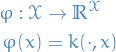
Let be an arbitrary set and a Hilbert space of real-valued functions on . The evaluation functional over the Hilbert space of functions is a linear functional that evaluates each function at a point ,

We say that is reproducing kernel Hilbert space if, for all in ,  is continuous at any in , or, equiavelently, if is a bounded operator on , i.e. there exists some such that

While this property for ensure both the existence of an inner product and the evaluation of every function in at every point in the domain. It does not lend itself to easy application in practice.
A more intuitive definition of the RKHS can be obtained by observing that this property guarantees that the evaluation functional can be represented by taking the inner product of with a function  in . This function is the so-called reproducing kernel of the Hilbert space from which the RKHS takes its name.
The Riesz representation theorem implies that for all there exists a unique element of with the reproducing property

Since is itself a function in , it holds that for every in there exists a  s.t.
s.t.
This allows us to define the reproducing kernel of as a function  by
by
From this definition it is easy to see that is both symmetric and positive definite, i.e.
for any  ,
,  and some
  .
.
- RKHS in statistcal learning theory
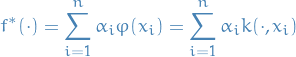
The representer theorem states that every function in an RKHS that minimizes an empirical risk function can be written as a linear combination of the kernel function evaluated at the training points.
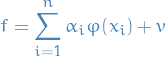
Let
 be a nonempty set and a postive-definite real-valued kernel on
  with corresponding RKHS .
Given a training sample
 , a strictly monotonically increasing real-valued fuction
  , and a arbitrary emipirical risk function
  , then for any
  satisfying
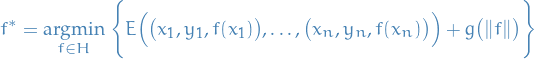
 admits a representation of the form
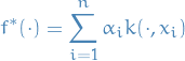
where
 for all
  and, as stated before, is the kernel on the RKHS .
Let
(so that
 is itself a map
  )
)
Since
is a reproducing kernel, then

where
 is the inner product on .
Given any
 , one can use the orthogonal projection to decompose any
  into a sum of two functions, one lying in the
  and the other lying in the orthogonal complement:
where
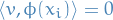 for all
  .
.
The above orthogonal decomposition and the reproducing property of
show that applying to any training point  produces
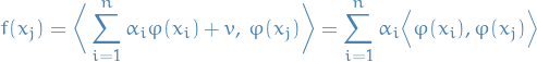
which we observe is independent of
. Consequently, the value of the empirical risk in defined in the representer theorem above is likewise independent of .
For the second term (the regularization term), since
is orthogonal to summand-term and is strictly monotonic, we have
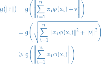
Therefore setting
 does not affect the first term of the empirical risk minimization, while it strictly decreasing the second term.
Consequently, any minimizer
of the empirical risk must have , i.e., it must be of the form
which is the desired result.
This dramatically simplifies the regularized empirical risk minimization problem. Usually the search domain
for the minimization function will be an infinte-dimensional subspace of  (square-integrable functions).
But, by the representer theorem, we know that the representation of
 reduces the original (infinite-dimensional) minimization problem to a search for the optimal n-dimensional vector of coefficients
  for the kernel for each data-point.
Theorems
Let  , then
Let . Consider the following polynomial

where we've used the fact that  for
for  .
.
Since it's nonnegative, it has at most one real root for , hence its discrimant is less than or equal to zero. That is,
Hence,
as claimed.
Let be a metric space.
- A sequence in can have at most one limit.
- If converges to and
 is any subsequence of , then
  converges to as
 - Every convergence sequence in is bounded
- Every convergence sequence in is Cauchy
Let . Then  as if and only if

Let . Then is closed if and only if the limit of every convergent sequence  satisfies
A set is open iff it equals its interior ; a set is closed iff it equals its closure .
Let be a metric space and let . Then, is dense if and only if  .
.
Any compact set must be closed and bounded.
The converse is not necessarily true (Heine-Borel Theorem addresses when this is true).
Bounded:
 is compact implies that
  s.t.
s.t.
where
 .
.
Let be a separable metric space which satisfies the Bolzano-Weierstrass Property and  . Then is compact if and only if it is closed and bounded.
Observe that
is closed and bounded.
 is compact if and only if
  .
.
Suppose  . Idea is cto construct
  of unit vectors s.t.
Example: continuous functions
![$\big( C([0, 1]), \norm{\cdot}_{L^\infty} \big)$](../../assets/latex/analysis_f10d5d78c04b9ac1817e46272c1ff549f3bac865.png) is a Banach space.
is a Banach space.
What are the compact sets ![$K \subseteq C([0, 1])$](../../assets/latex/analysis_2e16dc359c627731048e8518b88cef2cb0f48f17.png) ?:
?:
- is compact if and only if is closed, bounded AND "something something" (what is it?)
Continuity and limits of functions
Let where and  are metric spaces.
Then  if and only if for every we have

Or equivalently, if is continuous on ,

Connected sets
Let be a metric space.
- A pair of nonempty open sets
 is said to separate if and only if
  and
and 
- is said to be connected if and only if cannot be separated by any pair of open sets

Loosely speaking, a connected space cannot be broken into smaller, nonempty, open pieces which do not share any common points.
Let be a metric space, and .
are said to separate if and only if:
 (non-empty)
is connected if and only if it cannot be separated by any .
A subset  is connected if and only if is an interval
A subset of a metric space is path-connected if for every  there is a continuous function (path)
 ![$\phi: [0, 1] \to E$](../../assets/latex/analysis_6184738782cb70109b33fdf41748761949272ac4.png) such that
such that

Let be a metric space, and  .
.
If is path-connected , then is connected.
Stone-Weierstrass Theorem
Notation
- is a metric space
- denotes a algebra in


Goal
The goal of this section is to answer the following question:
Can one use polynomials to approximate continuous functions on an interval ?
Stuff
Let be a metric space.
A set is a said to be a (real function) algebra in if and only if
- If
 , then
  and both belong to
 - If
 and , then
A subset of is said to be (uniformly) closed if and only if for each sequence  that satisfies
  as , the limit function belongs to .
A subset of is said to be uniformly dense in if and only if given and  there is a function
  such that
  .
.
A subset of separates points of if and only if given  with
with
Stone-Weierstrass Theorem
Suppose that is a compact metric space.
If is an algebra in that separates points of and contains the constant functions, then is uniformly dense in .
This is HUGE. It basically says that on any compact metric space, we can approximate any continuous function arbitrarily well using only the constants functions and some functions which separates points in the metric space!
You know what space satisfies this? Space of all polynomials!
Q & A
DONE Alternative definition of compact; consequences?
What's the difference between the definition of compactness and the following:
A set is compact if for every subset there exists a finite covering .
Is there any difference; and if so, what are the consequences?
Answer
Yes, there is a difference.
In our new definition we're only saying that the EXISTS some finite covering, while the proper definition is sort of saying that all coverings of does in fact contain a finite covering, a sort of "the lowest common denominator covering has to be finite, and each of these coverings do in fact have this".
Fixed Point Theory
Differential Equations
Notation
Stuff
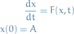
In this section we're considering the large class of ODEs of the form
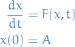
there will exists a unique solution  for sufficiently small.
To ensure the existence of a unique solution, we need to consider the following:
Suppose  and
and  . Also suppose and
  and
and
![\begin{equation*}
F: [A - \rho, A + \rho] \times [-r, r] \to \mathbb{R}
\end{equation*}](../../assets/latex/analysis_c9ddc35a4b00aa728286a03ed85db37856e4c4a5.png)
is continuous.
Further, suppose that for all ![$x, y \in [A - \rho, A + \rho]$](../../assets/latex/analysis_175d5c1c72ff749ff44e2ce3e0131678303ec09c.png) and
and ![$t \in [-r, r]$](../../assets/latex/analysis_3adcafac40b791f1895983b733f8e2180cc1de2e.png) there exists such that
there exists such that

Due to Mean Value Theorem, if  exists and is continuous on
 ![$[A - \rho, A + \rho] \times [-r, r]$](../../assets/latex/analysis_65edd9aed40242497d2e71bf8dc765b9fc2019fe.png) then the above is satisfied.
then the above is satisfied.
Suppose  satisfies a Lipschitz condition as above. Then there exists an
  such that the ODE
has a unique solution for  .
.
Exercises
From the notes
A contraction is continuous
A contraction is continuous.
Let , and let be a contraction. Now, for the sake of contradiction, suppose is discontinuous at some point .
Due to being a contraction, then for any two points  we have
where  . Since is arbitrary we can let be such that
Clearly,
Thus,

Which implies,
But this is only true if and only if is continuous; hence we have our contradiction.
TODO Exercise 1
Suppose is a contraction mapping.
If

then any fixed point will be unique, whether or not is complete.
Further, show that if is not complete, then a fixed-point does not necessarily exist.
Let be a metric space.
For the first part of our claim, suppose the mapping satisfies

Then clearly is a contraction, since we can always choose such that

due to the interval  being dense in .
Now, for the sake of contradiction suppose there exists two different fixed-points,  . Then, from the property above of , we have
But, since  and
and  are fixed-points, we have
Hence, the above inequality implies
Which clearly is a contraction, hence if there exists a fixed-point of , then that is a unique fixed-point.
Now, for the second part of the claim,
PROBABLY EXIST SOME COUNTER-EXAMPLE THAT I CAN'T THINK OF. SOME SUCH THAT THIS IS NOT THE CASE.
TODO Exercise 2
Let be a metric space which is not complete. Then there exists contractions with no fixed point.
Probably some counter-example I can't think of.
TODO Exercise 3
Note taken on
Regarding the previous note, could we not have
which for even
we would still have  be a contraction mapping, but for odd it would not be! Therefore I believe it's reasonable to assume that they mean for any .
- Note taken on
But alone does not imply that
  since
since  , could be
  , hence there needs to be something else which ensures this implication. That is, if the claim is supposed to be true for any , then yeah, this implication would definitively hold, but I'm not sure that is what they mean
 - Note taken on
being a contraction in a complete metric space => is a contraction in a complete metric space => has a unique fixed point in this space: NOPE! We can have fixed points without the function being a contraction, also being a contraction does not in fact imply that is a contraction! See Exercise 4 for a counter-example.
Let be a complete metric space, and suppose is such that

is a contraction. Then has a unique fixed point.
As proven in the first part of Exercise 1 we know that any contraction  has a unique fixed point when is a complete metric space. Thus, we know that there exists some such that
If we assume the claim is supposed to hold for any , and not a specific arbitrary , then the above implies

Further, if was not unique, then

for some  , but this implies that has another fixed point, which we know cannot be.
Hence, if is a contraction, then has a unique fixed point.
TODO Exercise 4
Note taken on
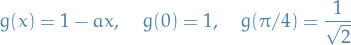
Maaaybe you can build some argument by creating two linear functions and
and  which intersect
  at a single point
  , and such that
![\begin{equation*}
g_1(t) = g_2(t) = \cos t, \quad g_1(x) \le \cos x, \quad g_2(x) \ge \cos x, \quad x \in [0, t]
\end{equation*}](../../assets/latex/analysis_8bd7d58244fdab167992a15c695ddb8a35aa2571.png)
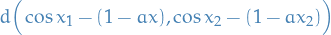
Basically, consider two functions for which we can easily compute the effect of
for two points and on the distance between them  which we can clearly tell has the property that
  , buuut I'm not going to bother spending time on this now.
Note taken on
But, if we can show that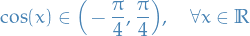
and then

we're good!
Note taken on
I was wondering if we can use some function on the interval
  which is defined such that
which also has the property that
 for , and then we potentially compute the distance of the difference between these functions to obtain some upper-bound on which related to
  .
.
Doesn't seem to work very well though
- Note taken on
Technically we only need to prove that is a contraction mapping on the open interval
  , since for not in this interval,
  will lie in the interval specified before.
 is not a contraction, but
  is a contraction.
Further, this implies that there is a unique solution in to the equation

Clearly  is not a contraction, since
which implies
and
Hence,

NOW PROVE THAT  IS A CONTRACTION MAPPING YAH FOOL
Fourier Series
Notation
Definition
Let be integrable on ![$[- \pi, \pi]$](../../assets/latex/analysis_8ccfa4861271a40956d9a5fddb99884ce26ce0c6.png) .
.
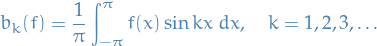
The Fourier coefficients of are numbers
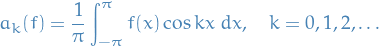
and
Let be integrable on and let  be a nonnegative integer.
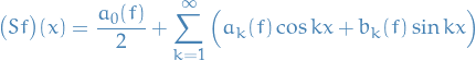
We define the Fourier series of as the trigonometric series
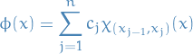
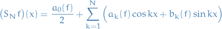
and the partial sum of  of order to be the trigonometric polynomial defined
Kernels
Dirichlet kernel
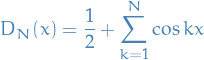
Let be nonnegative integer.
The Dirichlet kernel of order is the function defined
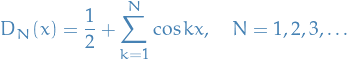
with the special case of  .
.
It turns out it can also be written as
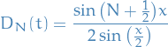
for all ![$x \in [-\pi, \pi]$](../../assets/latex/analysis_b6623df41ea8c5cec3380cab5139b04d7c35813a.png) and .
and .
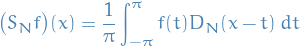
That is, we can write the N-th order Fourier partial sum as a convolution between and the Dirichlet kernel.
![\begin{equation*}
\begin{split}
\big( S_N f \big) (x) &= \frac{1}{2 \pi} \int_{-\pi}^{\pi} f(t) \ dt + \frac{1}{\pi} \sum_{k=1}^{N} \int_{-\pi}^{\pi} f(t) \Big( \cos kt \cos kx + \sin kt \sin kx \Big) \ dt \\
&= \frac{1}{\pi} \Bigg[ \int_{-\pi}^{\pi} \Bigg( \frac{1}{2} + \sum_{k=1}^{N} \cos \Big( k (x - t) \Big) \Bigg) f(t) \ dt \Bigg]
\end{split}
\end{equation*}](../../assets/latex/analysis_0e6754c427298fb24ff98648707806eab0cc0fc3.png)
where we've brought the intergrals together and used the trigonometric identity

Finally remembering that
We see that the above expression is simply
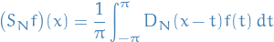
as claimed.
Suppose that ![$f_N: [-\pi, \pi] \to \mathbb{R}$](../../assets/latex/analysis_9bb56fef7a0123394a78936fbe764d04b2c81711.png) is integrable and that
is integrable and that  uniformly on . Then,

as  uniformly in .
We know that  such that
![\begin{equation*}
\forall N \ge N_0 \quad \implies \quad |f_N - f| < \varepsilon, \quad \forall x \in [-\pi, \pi]
\end{equation*}](../../assets/latex/analysis_e2183e22e7f2ea8b02cf5266ede72113418c7763.png)
Then we have,
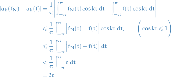
I.e. we can make the difference between the coefficients as small as we'd like, hence

The very same argument holds for .
Fejér kernel
The Fejér kernel of order is the function defined
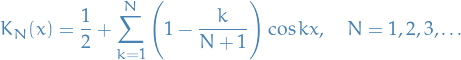
with the special case of .
Functional Analysis
Notation
 is the fields we'll be using
"Small Lp" space:
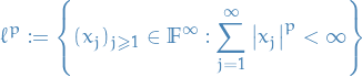
Let
 be a measure space and
  , then

denotes the set of all measurable functions
on such that  and the values of are real numbers, except possibly on a set of measure
  .
.
Lp space:
![\begin{equation*}
L^p = \left\{ f: [0, 1] \to \mathbb{R} : \norm{f}_{L^p} < \infty \right\}
\end{equation*}](../../assets/latex/analysis_07d28570438667e9ce005288e62357a7bbad4cde.png)
where
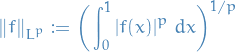
Or more accurately,

where
 denotes the equivalence classes of the equivalence relation

- NLS means normed linear spaces
Theorems
Inequalities
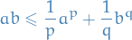
Let  such that
  . Then
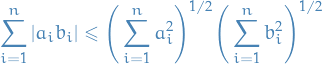
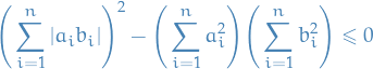
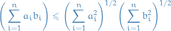
For any two sequences  and
and 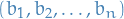 of nonnegative numbers, we have
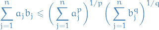
for any  where
where  is the conjugate exponent of , i.e.
Observe that this aslo includes  and
and  !
!
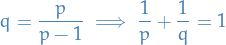
For and :

From Hölders inequality we have
where  . Finally, letting
  and
and  , we get

And taking both sides to the power of :

as wanted.
For any two elements  and
and  of
of  , we have
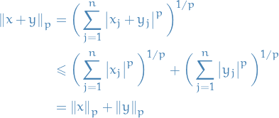
for any .
Mercer's theorem
Let ![$K: [a, b]^2 \to \mathbb{R}$](../../assets/latex/analysis_9094fa2e92b0f7404e1360129684d05a5019f3c5.png) be a symmetric continuous function, often called a kernel.
be a symmetric continuous function, often called a kernel.
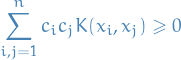
is said to be non-negative definite (or positive semi-definite) if and only if
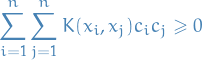
for all fininte sequences of points ![$x_1, \dots, x_n \in [a, b]$](../../assets/latex/analysis_df408ebd5b590a92452fc6df4e55a0f880cc7ffc.png) and all choices of real numbers
and all choices of real numbers  .
.
We associate with a linear operator ![$T_K: L^2([a, b]) \to L^2([a, b])$](../../assets/latex/analysis_5f9dfc4f9e9bcce9ac9d7c164cb268f6a8bc8c39.png) by
by
![\begin{equation*}
\big( T_K \varphi \big) (x) = \int_{a}^{b} K(x, s) \varphi(s) \ ds, \quad \varphi \in L^2([a, b])
\end{equation*}](../../assets/latex/analysis_e0221b304336728d74b7277973b37066aeef26fc.png)
The theorem then states that there is an orthonormal basis  of
of ![$L^2([a, b])$](../../assets/latex/analysis_46dd0ac7af731cb49a65fdba69a9f752782dd5f8.png) consisting for eigenfunctions of
consisting for eigenfunctions of  such that the corresponding sequence of eigenvalues
  is nonnegative.
The eigenfunctions corresponding to non-zero eigenvalues are continuous on and has the representation
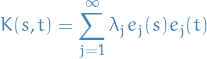
where the convergence is absolute and uniform.
There are also more general versions of Mercer's thm which establishes the same result for measurable kernels, i.e.  on any compact Hausdorff space .
Banach spaces
A norm on a vector space  over
over  (
( or
or  ) is a map
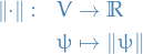
with the following properties:
- For all
 ,
,  , with equality if and only if
- For all and
 , we have
For all
 , we have

If  is a norm on , then we can define a metric on by setting
 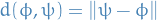 .
.
A normed vector space is said to be a Banach space if it is complete wrt. the associated metric.
A Banach space is said to be separable if it contains a countable dense subset.
Let  be a normed space and
  a Banach space.
Suppose  is a dense subset of and that
  is a bounded linear operator.
Then there exists a unique bounded linear map  such that

where  denotes the restriction of
  to the subspace .
Furthermore, the norm of equals the norm of .
Suppose that is a Banach space and a normed vector space.
For any linear map  , let
, let  denote the set of pairs
  in
in  such that
  .
.
If the graph of is a closed subset of , then is bounded.
Examples
Equip ![$C \big( [0, 1] \big)$](../../assets/latex/analysis_8a6793132a8063104c20b7b52560ffd95a9ff44f.png) with the norm
with the norm
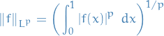
Then,

Metric space structure on NLS
Let  is a NLS of
  is a subspace.
If is open, then  .
.
Clearly  , hence
  there exists

Observe that  if and only if
  for some
  .
.  by definition of a subspace, and reverse is
  which implies that
  .
.
Cosnider  since
since  . Then,

So basically, since a linear space is closed under scalar multiplication, any open subspace must contain any scaling of  , hence it must contain the entire space.
Let be a NLS with .
Then is closed.
Completion of NLS
Notation
- denotes a NLS which is not necessarily complete
 denotes the completion of
 Set of Cauchy sequences in
:
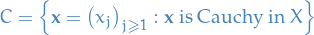
Stuff
- Formal procedure to "fill holes" in an NLS, i.e. making non-complete NLS (NLS for which Cauchy sequences does not necessarily converge), well, complete!
- Observe that is dense in the completion of , i.e.

- Let
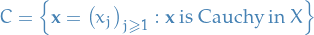 .
.
Let
 on be the equivalence relation such that

Let be a Banach space, and let be a subspace.
Then  is a Banach space if and only if is closed.
Suppose is closed. Let  be Cauchy. Then is Cauchy in .
And since is closed, contains all its limit points, hence all convergent sequences in converges to a point in , i.e. is Banach.
be Cauchy. Then is Cauchy in .
And since is closed, contains all its limit points, hence all convergent sequences in converges to a point in , i.e. is Banach.
 . Suppose is a Banach space.
Let s.t. for some .
Note that is Cauchy, and since is Banach, there exists an
. Suppose is a Banach space.
Let s.t. for some .
Note that is Cauchy, and since is Banach, there exists an  s.t.
s.t.  as . Then

Hence,  , and is closed.
Let  and
and  be two normal linear spaces.
- A linear map
 is said to be an isometry if
  for all .
 - We say and are isometrically isomorphic if there exists an isometry from to .
- Note that
 is automatically a surjective isometry.
- Note that
- The Banach space completion of is a pair, consisting of a Banach space and an isometry s.t.
 is a dense subspace of .
Let  and
and  be two completions of .
Then and are isometrically isomorphic.
Let be an NLS.
Then there exists a unique a Banach space completion of .
Let
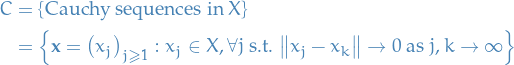
Equivalence relation
on

Let
 , and define
![\begin{equation*}
\begin{split}
T: \quad & X \to \tilde{X} \\
& x \mapsto Tx = [\mathbf{x}]
\end{split}
\end{equation*}](../../assets/latex/analysis_a8126eee401a3f468abb9bf8297f2188f0603fdd.png)
Observe that
![\begin{equation*}
\mathbf{y} \in [\mathbf{x}] \iff \norm{y_j - x} \to 0
\end{equation*}](../../assets/latex/analysis_ec1a86a40c65eac83c10217f78c6202c0a211e9e.png)
i.e. all sequences which converges to
.
Equip
 a vector space structure, i.e. addition
![\begin{equation*}
[\mathbf{x}] + [ \mathbf{y}] = [\mathbf{z}], \quad \mathbf{z} = \big( x_j + y_j \big)_{j \ge 1} \in C
\end{equation*}](../../assets/latex/analysis_a501bd7d7765d7b68308d5a782b2aa6aa7fb5140.png)
and scalar multiplication
![\begin{equation*}
\lambda [\mathbf{x}] = [\lambda \mathbf{x}]
\end{equation*}](../../assets/latex/analysis_568bc53761573745d90260e1166e155ce83cb382.png)
Equip
with a norm 

Observe that

By completion of the underlying field
,  is Cauchy and thus converges. Hence the above norm is defined
Need to check that this is well-defined:
![\begin{equation*}
y \in [\mathbf{x}] \iff \norm{y_j - x_j} \to 0 \iff \lim_{j \to \infty} \norm{y_j} = \lim_{j \to \infty} \norm{x_j}
\end{equation*}](../../assets/latex/analysis_56e45eaa2511a52884243f13f496b6056c05c22e.png)
 is a Banach space
Then
 is a linear map, then
![\begin{equation*}
\norm{T \mathbf{x}}_{*} = \norm{[\mathbf{x}]}_{*} = \lim_{j\to \infty} \norm{x_j} = \norm{x}
\end{equation*}](../../assets/latex/analysis_9e9812f841499e9885f9ae2068f73891d2ce5f09.png)
Finally, one can show that
is dense in , hence we have our Banach space completion.
Example
Let  be a subspace.
 , i.e.
  is closed in
  .
.
Let  , thus
  . Then

for some  .
.
We then need to show that  or
or  as
as  . or
. or

Given . Then  s.t.
s.t.  .
But
.
But  implies
So for  ,
,

So basically, show that a sequence of sequences  converge to some sequence , thus contains all it's limit points, hence is closed.
Consider the NLS ![$\big( C([0, 1]), \norm{\cdot}_{L^p} \big)$](../../assets/latex/analysis_0beb12faa8264445971d8af40206cf4e849a84ad.png) for
for  .
.
Let
![\begin{equation*}
S = \left\{ f \in C([0, 1]) : f(0) = 0 \right\}
\end{equation*}](../../assets/latex/analysis_a058cbfca87a98d53838bdd80011bcdcc53f6576.png)
Then is not closed, but is dense in ![$C([0, 1])$](../../assets/latex/analysis_d0a786318a6f7e61dfb7af9b501295ff0c1a81b9.png) , i.e.
, i.e.
![\begin{equation*}
\overline{S} = C([0, 1])
\end{equation*}](../../assets/latex/analysis_1e17bfffa65218879509d202ecbf5f47d6153b12.png)
Let
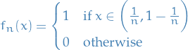
Then  , therefore
  .
But
.
But  , but
, but  , hence does not contain all of its limit points, i.e. is not closed, proving our first claim.
Now suppose that ![$f \in C([0, 1])$](../../assets/latex/analysis_795511f38a674f2eca972b1e89f37e957086b05e.png) . We now want to show that
. We now want to show that  such that and .
TO THIS.
Equivalence of norms
- We'll be referring to norms as equivalent if the induced norms are strongly equivalent metrics
Two norms  and
and  on are said to be equivalent if there is a constant s.t.

This does in fact define an equivalence relation on norms.
Hilbert spaces
Let be a  and
and  its dual space.
Then the map
its dual space.
Then the map

Then is isometric isomorphism.
If  is a bounded linear functional, then there exists a unique
  such that

Furthermore, the operator norm of  as a linear functional is equal to the norm of
  as an element of
  .
.
 and
and  s.t.
s.t. 
Assume
 and consider

 is closed (
 cont.) and subspace ( linear) of . Then

since
.
- But
 implies there exists nonzero
  .
. Take

and check

Basis in Hilbert spaces
Orthogonal decomposition
If  , then
For any seminorm defined by a semi-inner product and any  ,
,

For any inner product space  , and any Hilbert subspace
  , and
, and  there is a unique representation

with  and
and  .
.
Idea:
- Prove existence of orthogonal decomposition
- Proof by contradiction
- Consider a lower-bound on the distance between
 for
for  , and then show that this is violated if
  , i.e. the "rest" of is not in
  .
.
- Prove uniqueness
Let

Then let  such that
  and
and  .
.
Then, by lemma:parallelogram-law we have

thus,
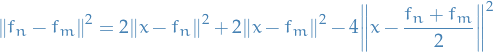
By completeness of , we know that  . Further, observe that
  , thus by def. of ,
Thus, as  , we have
  for some .
Now let  . Then

by continuity of  and the fact that
  and .
and .
Further, suppose that for some . Let
and  .
.
Then we observe that

Substituting back in our epxression for :

The last term is simply  , thus

For sufficiently small , the term dominates which implies that
for  .
.
This clearly contradicts our definition of , hence we have the proof of decomposition existence by contradiction.
For uniqueness of the decomposition, we simply observe that if also  for some
  and
and  , then
thus

which implies  and
and  .
.
Many functions in  of Lebesgue measure, being unbounded, cannot be integrated with the classical Riemann integral. Therefore spaces of Riemann integrable functions would not be complete in the norm, and the orthogonal decomposition would not apply to them.
Another victory for good ole' Lebesgue!
Orthonormal sets and bases
A set  in a semi-inner product space is called orthonormal if and only if
For any orthonormal set  and ,
and ,
If  is an orthonormal set in , and
  , where
and
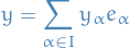
Then 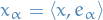 and
and 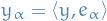 for all
  .
.
Furthermore,
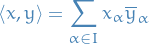
For any Hilbert space , any orthonormal set and any  , then
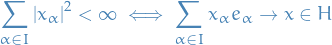
 : Follows from Bessel's inequality and Parseval-Bessel equality, since we have
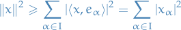
where the first equality is from Bessel's inequality and the second from Parseval-Bessel equality.
: For each  choose a finite set
  such that
  increases with and
Then
is a Cauchy sequence, hence converges to some since is complete.
Then the net of all partial sums converges to the same limit, concluding our proof.
Let be any inner product space and  be any linearly independent sequenec in .
Then there is an orthonormal sequence  in s.t. for each ,
  and
and  have the same linear span.
- Side-note on why Hilbert space > Banach space when talking about bases
In any vector space
, a Hamel basis is a set such that every  can be written uniquely as

with only finitely many
 .
.
So, Hamel basis is an algebraic notion, which does not relate to any topology on
.
In a separable Banach space
, a Schauder basis is a sequence  such that for every ,
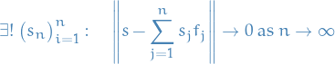
It is possible to find a Schauder basis in the "most useful" separable Banach spaces, but Schauder bases may not be conditional bases, and in general it may be very hard to find unconditional bases.
- Orthonormal basis for Hilbert space
Coming up with a basis for an infinite-dimensional space comes down to constructing a sequence of orthonormal vectors
 by taking some vector for which the projection
  , i.e. all of
  does not lie in
  .
.
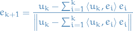
Then we prove that this gives us a space which is dense in the "parent" space.
More concretely, let
 and
and  be defined by choosing some
  such that
  , i.e.
  , and
, and
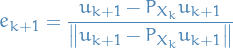
Every Hilbert space has an orthonormal basis.
If a collection of orthonormal sets is linearly ordered by inclusion (a chain), then their union is clearly an orthonormal set.
Thus by Zorn's lemma, let
be the maximal orthonormal set.
Take any
. Let
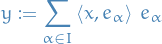
where the sum converges by Bessel's inequality and Riesz-Ficher theorem.
If
, we are done. Otherwise, then  for all , so we can adjoin a new element

contradicting the maximality of the orthonormal set.
Every Hilbert space is isometric to a space
 for some set .
Let
 be an orthonormal basis for .
Then
 takes into by Bessel's inequality.
This function preserves inner products by the Parseval-Bessel equality. It is onto
by the Riesz-Fischer theorem, concluding our proof.
For any inner product space
, an orthonormal set is an orthonormal basis of if and only if its linear span is dense in .
Let
 be a orthonormal sequence in a Hilbert space .
The following are equivalent:
If
s.t.  for all
  , then

In other words, the sequence
 is a maximal orthonormal family of vectors.
Span of
 is dense in
Unique convergence
then
Inner product on basis
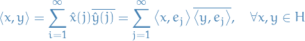
The norm
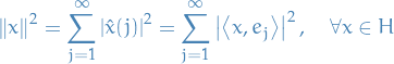
If one of these statements hold (and thus all of them hold), we say
is an orthonormal basis of .
 : Idea is that
  implies
  as a subspace is simply
  , hence the closure is dense in .
Suppose
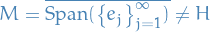 .
.
Then since
, we have  and so
  s.t.
s.t.  and for all . But this is a contradiction wrt. , hence we have our proof.
 : Let and since
 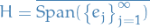 .
.
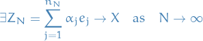
Set
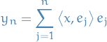
We make the following observations:
 and
and 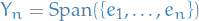 .
.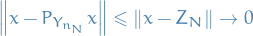 as
which tells us that a particular subsequence converges.
as
which tells us that a particular subsequence converges. we have
  ,
,
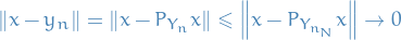
as
, since  . Which tells us that all possible subsequences converge.
Therefore
 .
.
 :
:
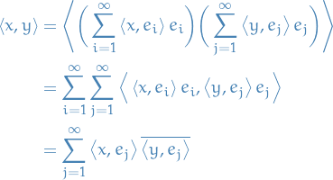
were we have used the interchanging of limits on multiple occasions, and in the final equality used the orthogonality of the
 .
.
 : Apply 4 with .
 : Otherwise we would have extra terms for the norm, rather than just the "Fourier" coefficients → contradiction.
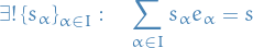
Bounded Linear Operators
Notation
- be linear operator and and are normed linear spaces
 be vector space of bounded linear operators from to .
- $T ∈
Stuff
Let be linear operator and and are normed linear spaces.
Then the following are equivalent
- is continuous on all of
- is continuous at

- is bounded
 is seen by observing that for a sequence we have

and so and  are equivalent.
 : Suppose is continuous at . Thus

Let  , and let
  and
and
So
which gives us
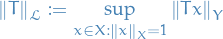
 .
.
If , then all linear maps are continuous.
Hence  .
.
 .
.
T is onto: let
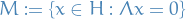
Then is a closed subspace of .
Suppose  , then we can decompose , then this implies there exists some nonzero
  .
.
Let and consider
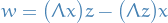
Then observe that

which implies that

which implies
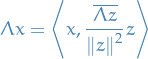
So for

Therefore,
or equiv,

and 
Let

is the subspace of finite rank operators.
Then for  and
and  , there exists
 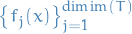 , i.e. constants which depend on (functions yo!) s.t.
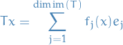
Then:
- is linear

 are linear for all
 - bounded / cont. are bounded / cont. for all
If  then
then  , i.e. the dual space of !
If is a Banach space, then is a Banach space.
Examples with  , i.e.
 for
for 
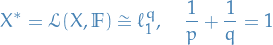
Fix  and define
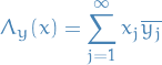
Then
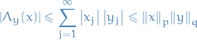
by Hölder's inequality. So  is bounded,

(remember we fixed ).
Hence  and
and  .
.
Letting
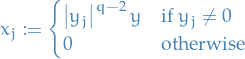
Then we attain the UB, and so we have equality.
We can then isometrically embed  into
into  . That is, we can show that for any
  , there exists
  s.t.
s.t.

Hilbert-Schmidt operators
Let  where
where  are separable Hilbert spaces.
We say that is a Hilbert-Schmidt operator if
The space of all such operators are denoted  with the norm defined
is a vector space and
but is not a closed subspace of  since
since
- Suppose
 be a ONB for and
  ONB for .
 Let
 then
then
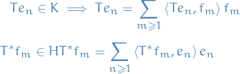
and
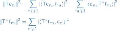
Thus,
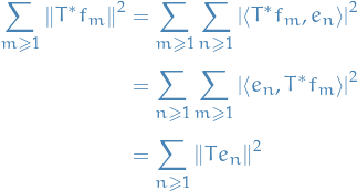
(switching sums we can always when all the terms are nonnegative).
- Hence, the definition of a Hilbert-Schmidt operator (also the norm
 ) is independent of the choice of ONB
Let
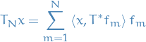
Then  is a FR operator.
 as then

since then 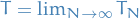 which would imply that contain the limit points of
  .
.
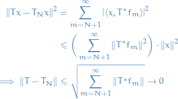
since i.e.
Example: kernel operators on ![$X = C([0, 1])$](../../assets/latex/analysis_8fe674cfb6c700fd8b70de8404a7c4713bc0d852.png)
Let ![$K \in C \big( [0, 1] \times [0, 1] \big)$](../../assets/latex/analysis_75b1515e39d70fb6460af8c4ac8706dc60ef8021.png) be what's called a kernel on and let
be what's called a kernel on and let
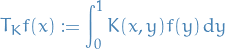
called a integral operator of .
Then
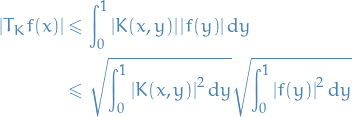
which implies that
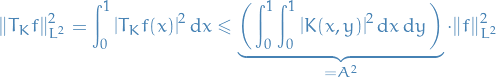
That is,
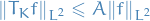
So is bounded and  .
.
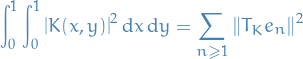
Let ![$H = L^2([0 , 1])$](../../assets/latex/analysis_afd7879552e1e7d31d0443706916f151a99a722f.png) be the completion of
be the completion of ![$\big( C([0, 1]), \left\langle \cdot, \cdot \right\rangle \big)$](../../assets/latex/analysis_e0d8221cd60c2ff589c97c3554435a7f82568a95.png) .
.
Consider the ONB defined by the Fourier coefficients  .
.
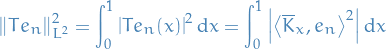
where
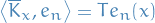
Summing over
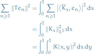
Compact operators
Notation
 denotes the space of compact operators
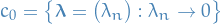 , i.e. denotes the set of all convergent sequences
Stuff
Let and be normed spaces and let  .
.
Then is said to be a compact operator if  is a compact subset of .
That is, is compact if the image of the unit closed ball is compact.
Recall that in finite-dimensional space, by Heine Borel, closed and bounded subsets are compact.
Hence finite-rank operators are always compact!
Suppose that is a normed space, is a Banach space and that  is a compact operator.
Suppose there is a s.t.  as . Then is compact.
 is a subspace of
 - If is a Banach space, then is closed (i.e. Theorem thm:limit-of-compact-operators-is-compact since it contains all its limit points)
- Supose are separable Hilbert spaces (thus there exist bases)
We have

- Though we will only prove

- Though we will only prove
- Let
 linear and
  be a ONB in , and assume
  since otherwise "containments" would be equality for all in the above.
 Furthermore, suppose
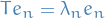
 iff
iff  and
and  , since
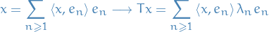
 iff
iff  and
and 
 iff
iff 
 iff
iff 
- iff
From this we get the above sequence of containments, since
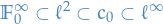
Spectral Theorem for Bounded Self-Adjoint Operators
Notation
- is the separable complex Hilbert space
Operator norm of
on is
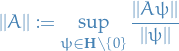
is finite.
- Banach space of bounded operators on , wrt. operator norm is denoted
 .
.  denotes the resolvent set of
  denotes the spectrum of
  denotes the projection-valued measure associated with the operator self-adjoint
 For any projection-vauled measure
and  , we have an ordinary (positive) real-valued measure
  given by
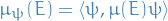
 is a map defined by
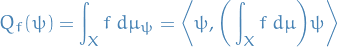
Spectral subspace for each Borel set

of
 defines a simultanouesly orthonormal basis for a family
  of separable Hilbert spaces
Properties of Bounded Operators
Linear operator
on is said to be bounded if the operator norm of
is finite.
Space of bounded operators on
forms a Banach space under the operator norm, and we have the inequality
for all bounded operators on
and .
For  , the resolvent set of , denoted is the set of all
  such that the operator
  has a bounded inverse.
The spectrum of , denoted by , is the complement in of the resolvent set.
For  in the resolvent set of , the operator
  is called the resolvent of at .
Alternatively, the resolvent set of can be described as the set of for which is one-to-one and onto.
For all , the following results hold.
- The spectrum of is closed, bounded and nonempty subset of .
- If
 , then is in the resolvent set of
Point 2 in proposition:hall13-quant-7.5 establishes that is bounded if is bounded.
Suppose satisfies  .
.
Then the operator  is invertible, with the inverse given by the following convergent series in :

For all , we have
![\begin{equation*}
\big[ \text{Range}(A) \big]^{\perp} = \text{ker}(A^*)
\end{equation*}](../../assets/latex/analysis_041fde8f7e956e923e6e23df6a01ead0a29b2641.png)
Spectral Theorem for Bounded Self-Adjoint Operators
Given a bounded self-adjoint operator , we hope to associate with each Borel set  a closed subspace
  of , where we think intuitively that is the closed span of the generalized eigenvectors for with eigenvalues in .
We would expect the following properties of these subspaces:
 and
and 
- Captures idea that generalized eigenvectors should span
- Captures idea that generalized eigenvectors should span
- If and are disjoint, then

- Generalized eigenvectors ought to have some sort of orthogonality for distinct eigenvalues (even if not actually in )
- Generalized eigenvectors ought to have some sort of orthogonality for distinct eigenvalues (even if not actually in
- For any and ,
If
 are disjoint and
  , then
- For any , is invariant under .
If
![$E \subset [\lambda_0 - \varepsilon, \lambda_0 + \varepsilon]$](../../assets/latex/analysis_bec5a95e47e8417fb8c1111121dd55490ad968ee.png) and
and  , then
Projection-Valued measures
For any closed subspace  , there exists a unique bounded operator such that
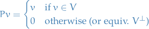
where  is the orthogonal complement.
This operator is called the orthogonal projection onto and it satisfies

i.e. it's self-adjoint.
One also has the properties

or equivalently,

Conversely, if is any bounded operator on satisfying  and
and  , then is the orthogonal projection onto a closed subspace , where

- Convenient ot describe closed subspaces of in terms of associated orthogonal projection operators
- Projection operator expresses the first four properties of the spectral subspaces; those properties are similar to those of a measures, so we use the term projection-valued measure
Let be a set and an  in .
in .
A map 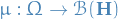 is called a projection-valued measure if the following properties are satisfied:
- For each
 ,
,  is an orthogonal projection
  and
and 
If
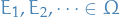 are disjoint, then for all
  , we have
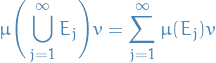
where the convergence of the sum is in the norm-topology on
.
- For all
 , we have
Properties 2 and 4 in of a projection-valued measure tells us that if  and
and  are disjoint, then
from which it follows that the range of  and the range of
  are perpendicular.
Let be a in a set and let  be a projection-valued measure.
Then there exists a unique linear map, denoted
from the space of bounded, measurable, complex-valued functions on into with the property that
for all and all .
This integral has the following properties:
For all
, we have
In particular, the integral of the constant function
is .
For all
, we have
Integration is multiplicative: For all
and , we have
For all
, we have
In particular, if
is real-valued, then  is self-adjoint.
By Property 1 and linearity, integration wrt. has the expected behavior on simple functions. It then follows from Property 2 that the integral of an arbitrary bounded measurable function can be comptued as follows:
- Take sequence
 of simple functions converging uniformly to
 - The integral of is then the limit, in the norm-topology, of the integral of the .
A quadratic form on a Hilbert space is a map  with the following properties:
 for all and
 the map
 defined by
![\begin{equation*}
\begin{split}
L(\phi, \psi) =& \frac{1}{2} \big[ Q(\phi + \psi) - Q(\phi) - Q(\psi) \big] \\
& - \frac{i}{2} \big[ Q(\phi + i \psi) - Q(\phi) - Q(i \psi) \big]
\end{split}
\end{equation*}](../../assets/latex/analysis_6085b0f14f4edf2b5f0f23825c97cba9ce1cc8de.png)
is a sesquilinear form.
A quadratic form is bounded if there eixsts a constant such that

The smallest such constant is the norm of .
If is a bounded quadratic form on , there is a unique such that

If  belongs to for all , then the operator is self-adjoint.
Spectral Theorem for Bounded Self-Adjoint Operators: direct integral approach
Notation
- is a measure on a of sets in
- For each
 we have a separable Hilbert space
  with inner product
- Elements of the direct integral are called sections

Stuff
There are several benefits to this approach compared to the simpler "multiplication operator" approach.
- The set and the function
 become canonical:
- The direct integral carries with it a notion of generalized eigenvectors / kets, since the space can be thought of as the space of generalized eigenvectors with eigenvalue .
- A simple way to classify self-adjoint operators up to unitary equivalence: two self-adjoint operators are unitarily equivalent if and only if their direct integral representations are equivalent in a natural sense.


Elements of the direct integral are called sections , which are functions on with values in the union of the , with property
We define the norm of a section by the formula
provided that the integral on the RHS is finite.
The inner product between two sections  and
and  (with finite norm) should then be given by the formula
Seems very much like the differential geometry section we know of.
- is the fibre at each point in the mfd.
- is the mfd.
First we slightly alter the concept of an orthonormal basis. We say a family  of vectors is an orthonormal basis for a Hilbert space if
and
This just means that we allow some of the vectors in our basis to be zero.
We define a simultanouesly orthonormal basis for a family of separable Hilbert spaces to be a collection of sections with the property that

Provided that the function  is a measurable function from into
 ![$[0, \infty]$](../../assets/latex/analysis_7c43cf12221cf82ea0f3550c49639ade5528d224.png) , it is possible to choose a simultaneous orthonormal basis
, it is possible to choose a simultaneous orthonormal basis  such that
is measurable for all and .
Choosing a simultaneous orthonormal basis with the property that the function

is a measurable function from into , we can define a section to be measurable if the function
is a measurable complex-valued function for each . This also means that the  are also measurable sections.
We refer to such a choice of simultaneous orthonormal basis as a measurability structure on the collection .
Given two measurable sections and , the function
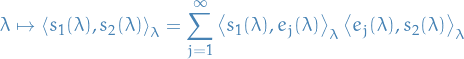
is also measurable.
Suppose the following structures are given:
- a measure space

- a collection
 of separable Hilbert spaces for which the dimension function is measurable
 - a measurability structure on
Then the direct integral of wrt. , denoted
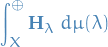
is the space of equivalence classes of almost-everywhere-equal measurable sections for which
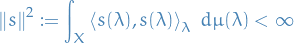
The inner product  of two sections and is given by the formula
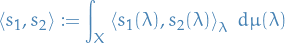
If is self-adjoint, then there exists a σ-finite measure on , a direct integral
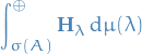
and a unitary map between and the direct integral such that
for all sections  .
.
Proofs
Notation
- with spectral radius
Stage 1: Continuous Functional Calculus
Stage 2: An Operator-Valued Riesz Representation Theorem
Let be a compact metric space and let  denote the space of continuous, real-valued functions on .
Suppose  is a linear functional with the property that
  is non-negative if is non-negative.
Then there exists a unique (real-valued, positive) measure on the Borel sigma-algebra in for which
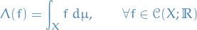
Observe that is a finite measure, with
where  is the constant function.
Continuous one-parameter groups
semigroup or strongly continuous one-parameter semigroup
A strongly continuous one-parameter semigroup on a Banach space is a map 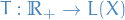 such that
 (i.e. identity operator on
  we have
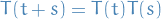
 we have
The first two axioms are algebraic, and state is a representation of a semigroup  , and the last axiom is topological and states that is continuous in the strong operator topology.
Infinitesimal generator
The infinitesimal generator of a strongly continuous semigroup defined by
whenever the limit exists.
The domain of , denoted  , is the set of for which the limit does exist; is a linera subspace and is linear on this domain.
The operator is closed, although not necessarily bounded, and the domain is dense in .
The storngly continuous semigroup with generator is often denoted by the symbol  , which is compatible with the notation for matrix exponentials.
Reproducing Kernel Hilbert Spaces (RKHSs)
Definitions
Let be a non-empty set, sometimes reffered to as the index set.
A symmetric function  is called a positive-definite kernel of if
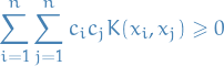
holds for any ,  , .
, .
Or more generally, for some field real or complex field  , a function
  is called a kernel on if there exists a
  and a map
  such that for all
  we have
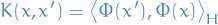
In machine learning context, you'll often see  be called a feature map and a feature space of .
The definition of a positive-definite kernel is equivalent to the following: A symmetric function is positive-definite if the matrix  with elements
![\begin{equation*}
\big[ k_{X X} \big]_{ij} = k(x_i, x_j)
\end{equation*}](../../assets/latex/analysis_552698d082ca0fca2447a0726f58904d0e84c322.png)
is positive semi-definite for any finite set  of any size .
This matrix  is often referred to as the kernel matrix or Gram matrix.
Note the swapping of order in the kernel and inner product above; this is only necessary in the case of a complex Hilbert space, where the inner product is sesquilinear:
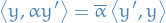
Examples of kernels
Let


Then a Gaussian RBF kernel or square exponential kernel is defined
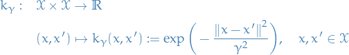
Let

The Matérn kernel is defined
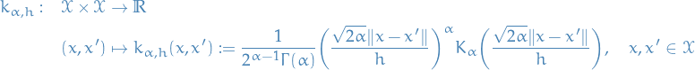
where
 is the gamma-function
 is the modified Bessel function of the second kind of order
- determines the scale
- determines the smoothness of the functions in the associated RKHS
- As increases, the functions get smoother
- As
If can be written as

for  , then the expression for the Matérn kernel reduces to a product of the exponentiated function and a polynomial of degree
  , which can be computed easily rasmussen2006gaussian:

For example  results in whats know as the Laplace or exponentiated kernel:
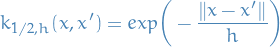
Gaussian RBF kernels can be obtained as limits of Matérn kernels for  , i.e. for a Matérn kernel
  with
with  being fixed, we have
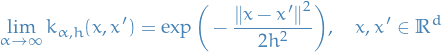
Let

Then a polynomial kernel is defined
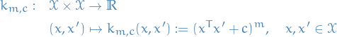
TODO Kernel embeddings
Exam prep
May 2017
1
c
If  uniformly continuous, and
  uniformly then is also uniformly continuous.
Given , find such that
In particular  ,
,
 is uniformly continuous, implies


Compactness
 , is closed and is compact, then is also compact.
Let  be any open cover of .

might not cover whole .  is open, therefore
is an open cover of . Thus, due to being compact, there exists a finite subcover of the above cover,

covers , then clearly  is a finite cover of , hence is compact, as claimed.
Proving connectedness of a set
- Best way to prove a set is connected is to check if it's path connected
- Best way to prove a set is not connected (disconnected), we use the definition of connectedness:
Find 2 open sets
such that

i.e. two sets such that the union covers
but they share no elements.