Measure theory
Table of Contents
Notation
 and
and  are used to denote the indicator or characteristic function
Definition
Motivation
The motivation behind defining such a thing is related to the Banach-Tarski paradox, which says that it is possible to decompose the 3-dimensional solid unit ball into finitely many pieces and, using only rotations and translations, reassemble the pieces into two solid balls each with the same volume as the original. The pieces in the decomposition, constructed using the axiom of choice, are non-measurable sets.
Informally, the axiom of choice, says that given a collecions of bins, each containing at least one object, it's possible to make a selection of exactly one object from each bin.
Measure space
If  is a set with the sigma-algebra
  and the measure
  , then we have a measure space .
Product measure
Given two measurable spaces and measures on them, one can obtain a product measurable space and a product measure on that space.
A product measure  is defined to be a measure on the measurable space
  , where we've let
  be the algebra on the Cartesian product
  . This sigma-algebra is called the tensor-product sigma-algebra on the product space, which is defined

A product measure is defined to be a measure on the measurable space satisfying the property

 and
and 
Let  be a sequence of extended real numbers.
The limit inferior is defined
The limit supremum is defined
Premeasure
Given a space  , and a collection of sets
  is an algebra of sets on if

- If
 , then
- If
 and
and  are in
  , then
Thus, a algebra of sets allow only finite unions, unlike σ-algebras where we allow countable unions.
Given a space and an algebra , a premeasure is a function ![$\lambda: \mathcal{A} \to [0, \infty]$](../../assets/latex/measure_theory_e17a0e8668dbd5fd1ed0e08c218ece154e7c2ed7.png) such that
such that

For every finite or countable collection of disjoint sets
 with
with  , if
, if  then
then
Observe that the last property says that IF this "possibly large" union is in the algebra, THEN that sum exists.
A premeasure space is a triple  where is a space, is an algebra, and a premeasure .
Complete measure
A complete measure (or, more precisely, a complete measure space ) is a measure space in which every subset of every null set is measurable (having measure zero).
More formally,  is complete if and only if

If  is a premeasure space, then there is a complete measure space
  such that

 we have
If  is σ-finite, then
  is the only measure on
  that is equal to on .
Atomic measure
Let  be a measure space.
Then a set  is called an atom if

and

A measure which has no atoms is called non-atomic or diffuse
In other words, a measure is non-atomic if for any measurable set  with
with  , there exists a measurable subset
  s.t.
s.t.
π-system
Let be any set. A family  of subsets of is called a π-system if

If
 , then

So this is an even weaker notion than being an (Boolean) algebra. We introduce it because it's sufficient to prove uniqueness of measures:
 be two finite measures on


Theorems
Jensen's inequality
Let
 be a probability space
 be random variable
![$c: \mathbb{R} \to (-\infty, \infty]$](../../assets/latex/measure_theory_0fbf01fc0b204736d63b072e13cefceee1e07280.png) be a convex function
Then
be a convex function
Then  is the supremum of a sequence of affine functions
for
 , with
  .
.
Then ![$\mathbb{E}[c(X)]$](../../assets/latex/measure_theory_a9eba1896bb741b60c40f7b709c13a7dfdf79cbf.png) is well-defined, and
is well-defined, and
![\begin{equation*}
\mathbb{E}[c(X)] \overset{a.s.}{\ge} a_n \mathbb{E}[X] + b_n
\end{equation*}](../../assets/latex/measure_theory_27722a1c52318e0443a664830effa0bb1a3503a3.png)
Taking the supremum over  in this inequality, we obtain
![\begin{equation*}
\mathbb{E}[c(X)] \ge c \big( \mathbb{E}[X] \big)
\end{equation*}](../../assets/latex/measure_theory_8c3280bc7d5e2fce41ec6d17771166c73ae27475.png)
be a convex function
Then  is the supremum of a sequence of affine functions
Suppose is convex, then for each point  there exists an affine function
  s.t.
s.t.
- the line
 corresponding to
  passes through
 - the graph of lies entirely above
Let  be the set of all such functions. We have
 because
  passes through the point
 beacuse all lies below
Hence
(note this is for each  , i.e. pointwise).
Sobolev space
Notation
- is an open subset of

 denotes a infinitively differentiable function
  with compact support
 is a multi-index of order
  , i.e.
Definition
Vector space of functions equipped with a norm that is a combination of  norms of the function itself and its derivatoves to a given order.
Intuitively, a Sobolev space is a space of functions with sufficiently many derivatives for some application domain, e.g. PDEs, and equipped with a norm that measures both size and regularity of a function.
The Sobolev space spaces  combine the concepts of weak differentiability and Lebesgue norms (i.e. spaces).
For a proper definition for different cases of dimension of the space  , have a look at Wikipedia.
Motivation
Integration by parst yields that for every  where
where  , and for all infinitively differentiable functions with compact support :
Observe that LHS only makes sense if we assume  to be locally integrable. If there exists a locally integrable function
  , such that
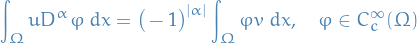
we call the weak -th partial derivative of . If this exists, then it is uniquely defined almost everywhere, and thus it is uniquely determined as an element of a Lebesgue space (i.e. function space).
On the other hand, if , then the classical and the weak derivative coincide!
Thus, if  , we may denote it by
  .
.
Example
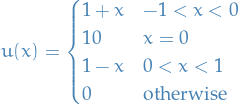
is not continuous at zero, and not differentiable at −1, 0, or 1. Yet the function
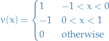
satisfies the definition of being the weak derivative of  , which then qualifies as being in the Sobolev space
  (for any allowed
  ).
).
Lebesgue measure
Notation
 denotes the collection of all measurable sets
Stuff
Given a subset  , with the length of a closed interval
 ![$I = [a,b]$](../../assets/latex/measure_theory_3fdf3f4bf882725c6261a1b413e5bc0b103e1281.png) given by
given by  , the Lebesgue outer measure
  is defined as

Lebesgue outer-measure has the following properties:
 Idea: Cover by
  .
.(Monotinicy)
 if
if  , then
Idea: a cover of
is a cover of .
(Countable subadditivity) For every set
 and every sequence of sets
  if
if  then
then
Idea: construct a cover of each
 ,
,  such that
  :
:
- Every point in is in one of the

- Every point in
Q: Is it possible for every  to find a cover
  such that
  ?
A: No. Consider
?
A: No. Consider  . Given
  , consider
  .
This is a cover of so
.
This is a cover of so  .
If
.
If  is a cover by open intervals of , then there is at least one
  such that
  is a nonempty open interval, so it has a strictly positive lenght, and
If  , then
![\begin{equation*}
\lambda^* \big( [a, b] \big) = \lambda^*([a, b)) = \lambda^* \big( (a, b] \big) = \lambda^* \big( (a, b) \big)
\end{equation*}](../../assets/latex/measure_theory_e6c6a70aa01d16ddfce344bbaedabbd1746e51f5.png)
Idea: ![$\big( a ,b \big) \subseteq [a, b]$](../../assets/latex/measure_theory_c7ddd35e2c2b0a06fa21ecb3622aa3c7a90f9cd9.png) , so
, so ![$\lambda^* \big( (a, b) \big) \le \lambda^* \big( [a, b] \big)$](../../assets/latex/measure_theory_a246293098d05d0199b421bc104c358809bd3568.png) .
For reverse, cover
.
For reverse, cover  by intervals giving a sum within
  .
Then cover
.
Then cover  and
and  by intervals of length
  .
Put the 2 new sets at at the start of the sequence, to get a cover of
.
Put the 2 new sets at at the start of the sequence, to get a cover of ![$[a, b]$](../../assets/latex/measure_theory_c9a1e8df376ecb942b106e02d3e6d1b417da2600.png) , and sum of the lengths is at most
, and sum of the lengths is at most  . Hence,
![\begin{equation*}
\lambda^* \big( (a, b) \big) \le \lambda^* \big( [a, b] \big) \text{ and } \lambda^* \big( [a, b] \big) \le \lambda^* \big( (a, b) \big)
\end{equation*}](../../assets/latex/measure_theory_e07a5a74202cf48119137eaee61040e633e6ac87.png)
If  is an open interval, then
  .
.
Idea: lower bound from  .
Only bounded nonempty intervals are interesting.
Take the closure to get a compact set. Given a countable cover by open intervals, reduce to a finite subcover.
Then arrange a finite collection of intervals in something like increasing order, possibly dropping unnecessary sets.
Call these new intervals
.
Only bounded nonempty intervals are interesting.
Take the closure to get a compact set. Given a countable cover by open intervals, reduce to a finite subcover.
Then arrange a finite collection of intervals in something like increasing order, possibly dropping unnecessary sets.
Call these new intervals  and let be the number of such intervals, and such that
i.e. left-most interval cover the starting-point, and right-most interval cover the end-point. Then
Taking the infimum,
The Lebesgue measure is then defined on the Lebesgue sigma-algebra, which is the collection of all the sets  which satisfy the condition that, for every

For any set in the Lebesgue sigma-algrebra, its Lebesgue measure is given by its Lebesgue outer measure  .
.
IMPORTANT!!! This is not necessarily related to the Lebesgue integral! It CAN be be, but the integral is more general than JUST over some Lebesgue measure.
Intuition
- First part of definition states that the subset is reduced to its outer measure by coverage by sets of closed intervals
- Each set of intervals covers in the sense that when the intervals are combined together by union, they contain
- Total length of any covering interval set can easily overestimate the measure of , because is a subset of the union of the intervals, and so the intervals include points which are not in
Lebesgue outer measure emerges as the greatest lower bound (infimum) of the lengths from among all possible such sets. Intuitively, it is the total length of those interval sets which fit most tightly and do not overlap.
In my own words: Lebesgue outer measure is smallest sum of the lengths of subintervals  s.t. the union of these subintervals completely "covers" (i.e. are equivalent to) .
If you take an a real interval ![$I = [a, b]$](../../assets/latex/measure_theory_f5678fa616e44d479ff19a74dbf6956a9abbbf8c.png) , then the Lebesge outer measure is simply
, then the Lebesge outer measure is simply  .
.
Properties
Notation
For
 and , we let
Stuff
The collection of Lebesgue measurable sets is a sigma-algebra.
Easy to see
 is in this collection:

Closed under complements is clear: let
be Lebesgue measurable, then

hence this is also true for
 , and so is Lebesgue measurable.
- Closed under countable unions:
Finite case:
 .
Consider
.
Consider  both Lebesgue measurable and some set .
Since
both Lebesgue measurable and some set .
Since  is L. measurable:

Since
 is L. measurable:

which allows us to rewrite the above equation for
 :
:

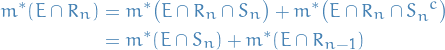
Observe that

By subadditivity:

Hence,
Then this follows for all finite cases by induction.
Countable disjoint case: Let
 , and . Further, let
 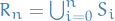 .
.
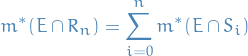
Hence
 is L. measurable. Thus,
Since the
are disjoint  and
and  :
:
Let
 and note that
  .
Thus, by indiction
.
Thus, by indiction
Thus,
Taking
 :
:
Thus,
 is L. measurable if the are disjoint and L. measurable!
- Countable (not-necessarily-disjoint) case:
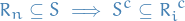
If are not disjoint, let
 and let
  , which gives a sequence of disjoint sets, hence the above proof applies.
Every open interval is Lebesgue measurable, and the Borel sigma-algebra is a subset of the sigma-algebra of Lebesgue measurable sets.
Want to prove measurability of intervals of the form  .
.
Idea:
- split any set into the left and right part
- split any cover in the same way
- extend covers by
 to make them open
 is a measure space, and for al intervals , the measure is the length.
Cantor set
Define
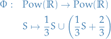
For , with  being identity, and

Let ![$E_0 = [0, 1]$](../../assets/latex/measure_theory_2841c9b582f2d0607515b04b91c33a1a58903197.png) and
and  . Then the Cantor set is defined

The Cantor set has a Lebesgue measure zero.
We make the following observations:
- Scaled and shifted closed sets are closed
 is a finite union of closed intervals and so is in the Borel sigma-algebra
- σ-algebras are closed under countable intersections, hence Cantor set is in the Borel σ-algebra
- Finally, Borel σ-algebra is a subset of Lebesgue measurable sets, hence the Cantor set is Lebesuge measurable!
Since Lebesgue measure satisfy  for any Lebesgue measurable set with finite measure and any with
  . Since Lebesgue measure is subadditive, we have for any

Since  , by induction, it follows that
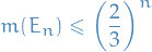
Taking the infimum of over  , we have that the Cantor set has measure zero:

Cardinality of the Cantor set
Let ![$x \in [0, 1]$](../../assets/latex/measure_theory_1abcf6a6ba0996351c652ec55b2a137f25774cfc.png) .
.
The terniary expansion is a sequence  with
with  such that
The Cantor set is uncountable.
We observe that if the first elements of the expansion for are in  , then
  . But importantly, observe that some numbers have more than one terniary expansion, i.e.
in the terniary expansion. One can show that a number  if and only if has a terniary expansion with no 1 digits. Hence, the Cantor set is uncountable!
One can see that if and only if terniary expansion with no 1 digits, since such an would land in the "gaps" created by the construction of the Cantor set.
Uncountable Lebesgue measurable set
There exists uncountable Lebesgue measurable sets.
Menger sponge
- Generalization of Cantor set to

Vitali sets
Let  if and only if
  .
.
- There are uncountable many equivalence classes, with each equivalence class being countable (as a set).
- By axiom of choice, we can pick one element from each equivalence class.
- Can assume each representative picked is in
![$[0, 1]$](../../assets/latex/measure_theory_68c8fa38d960e53d4308cbf1e65d04c66a554817.png) , and this set we denote
, and this set we denote 
Suppose, for the sake of contradiction, that is measurable.
Observe if , then there is a  and
and  s.t.
s.t. ![$q \in [-1, 1]$](../../assets/latex/measure_theory_e2a141e95f622cba27e76a7586a7befe39020eda.png) , i.e.
, i.e.
![\begin{equation*}
[0, 1] \subseteq \bigcup_{q \in [-1, 1] \cap \mathbb{Q}}^{} \Big( R + q \Big) \subseteq [-1, 2]
\end{equation*}](../../assets/latex/measure_theory_f79853c87366563f923b51372436ae537e0d78ed.png)
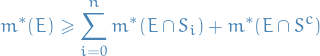
Then, by countable additivity
![\begin{equation*}
\begin{split}
m([0, 1]) &\le m \bigg( \bigcup_{q \in [-1, 1] \cap \mathbb{Q}}^{} R + q \bigg) \le m \big( [-1, 2] \big) = 3 \\
m([0, 1]) &\le \sum_{q \in [-1, 1] \cap \mathbb{Q}}^{} m (R + q) \le 3 \\
m([0, 1]) &\le \sum_{q \in [-1, 1] \cap \mathbb{Q}}^{} m (R) \le 3
\end{split}
\end{equation*}](../../assets/latex/measure_theory_10cc4bf4c4028ae61e6bec3e9a6df729d34e627e.png)
where we've used
![\begin{equation*}
m \bigg( \bigcup_{q \in [-1, 1] \cap \mathbb{Q}}^{} R + q \bigg) = \sum_{q \in [-1, 1] \cap \mathbb{Q}}^{} m (R + q) = \sum_{q \in [-1, 1] \cap \mathbb{Q}}^{} m (R)
\end{equation*}](../../assets/latex/measure_theory_4c878026d358487ad76ea895c4e45d05d969e74a.png)
Hence, we have our contradiction and so this set, the Vitali set, is not measurable!
There exists a subset of  that is not measurable wrt. Lebesgue measure.
Lebesgue Integral
The Lebesgue integral of a function  over a measure space
  is written

which means we're taking the integral wrt. the measure .

Special case: non-negative real-valued function
Suppose that  is a non-negative real-valued function.
Using the "partitioning of range of " philosophy, the integral of should be the sum over  of the elementary area contained in the thin horizontal strip between
  and
and  , which is just
Letting

The Lebesgue integral of is then defined by
where the integral on the right is an ordinary improper Riemann integral. For the set of measurable functions, this defines the Lebesgue integral.
Radon measure
- Hard to find a good notion of measure on a topological space that is compatible with the topology in some sense
- One way is to define a measure on the Borel set of the topological space
Let be a measure on the sigma-algebra of Borel sets of a Hausdorff topological space .
- is called inner regular or tight if, for any Borel set
 ,
,  is the supremum of
  over all compact subsets of
  of , i.e.
where
 denotes the compact interior, i.e. union of all compact subsets
  .
.
- is called outer regular if, for any Borel set , is the infimum of
 over all open sets
  containing , i.e.
where
 denotes the closure of .
- is called locally finite if every point of has a neighborhood for which is finite (if is locally finite, then it follows that is finite on compact sets)
The measure is called a Radon measure if it is inner regular and locally finite.
Suppose and  are two
  measures on a measures on a measurable space
  and is absolutely continuous wrt. .
Then there exists a non-negative, measurable function on such that
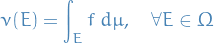
The function  is called the density or Radon-Nikodym derivative of wrt. .
If a Radon-Nikodym derivative of wrt. exists, then  denotes the equivalence class of measurable functions that are Radon-Nikodym derivatives of wrt. .
 is often used to denote
  , i.e. is just in the equivalence class of measurable functions such that this is the case.
This comes from the fact that we have
Suppose and  are Radon-Nikodym derivatives of wrt. iff
  .
.
The δ measure cannot have a Radon-Nikodym derivative since integrating  gives us zero for all measurable functions.
Continuity of measure
Suppose and are two sigma-finite measures on a measure space  .
.
Then we say that is absolutely continuous wrt. if

We say that and are equivalent if each measure is absolutely continuous wrt. to the other.
Density
Suppose and are two sigma-finite measures on a measure space and that is absolutely continuous wrt. . Then there exists a non-negative, measurable function on such that
Measure-preserving transformation
 is a measure-preserving transformation is a transformation on the measure-space if
Measure
A measure on a set is a systematic way of defining a number to each subset of that set, intuitively interpreted as size.
In this sense, a measure is a generalization of the concepts of length, area, volume, etc.
Formally, let be a  of subsets of .
Suppose ![$\mu: \mathcal{A} \to [0, \infty]$](../../assets/latex/measure_theory_beef385f676dedc4e7697f3bc64effffd9d7d3aa.png) is a function. Then is a measure if
is a function. Then is a measure if

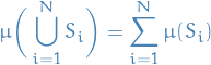
Whenever
 are pairwise disjoint subsets of in , then
- Called σ-additivity or sub-additivity
Properties
Let  be a measure space, and
  such that
  .
.
Then  .
.
Let

Then  , and by finite additivity property of a measure:

since  by definition of a measure.
If are  subsets of , then
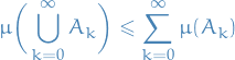
We know for a sequence of disjoint sets  we have
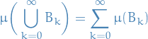
So we just let
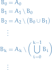
Then,
Thus,
Concluding our proof!
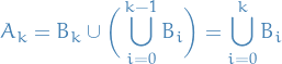
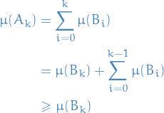
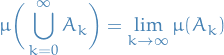
Let  be an increasing sequence of measurable sets.
Then
Let  be sets from some .
If  , then
Examples of measures
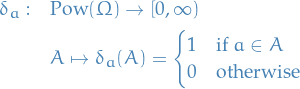
Let
- be a space

The δ-measure (at  ) is
) is
Sigma-algebra
Definition
Let be some set, and let  be its power set. Then the subset
  is a called a σ-algebra on if it satisfies the following three properties:

- is closed under complement: if
- is closed under countable unions: if

These properties also imply the following:

- is closed under countable intersections: if

Generated σ-algebras
Given a space and a collection of subsets  , the σ-algebra generated by
  , denoted
  , is defined to be the intersection of all σ-algebras on that contain , i.e.
where

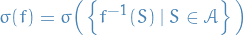
Let be a measurable space and  a function from some space to .
The σ-algebra generated by is
Observe that though this is similar to σ-algebra generated by MEASURABLE function, the definition differs in a sense that the preimage does not have to be measurable. In particular, the σ-algebra generated by a measurable function can be defined as above, where  is measurable by definition of being a measurable function, hence corresponding exactly to the other definition.
Let  and
and  be measure spaces and
  a measurable function.
The σ-algebra generated by is

![\begin{equation*}
\sigma \Big( \left\{ A \in \mathcal{A} \mid \exists c \in [- \infty, \infty): X^{-1} \big( (c, \infty] \big) = A \right\} \Big)
\end{equation*}](../../assets/latex/measure_theory_9164c3a0963daefb123e5c34ab8b2b62dc1220b5.png)
Let be a space.
If  is a collection of σ-algebras, then
  is also a σ-algebra.
σ-finite
A measure or premeasure space is finite if  .
.
A measure on a measure space  is said to be sigma-finite if can be written as a countable union of measurable sets of finite measure.
Example: counting measure on uncountable set is not σ-finite
Let be a space.
The counting measure is defined to be  such that
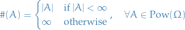
On any uncountable set, the counting measure is not σ-finite, since if a set has finite counting measure it has countably many elements, and a countable union of finite sets is countable.
Properties
Let be a of subsets of a set . Then

If
 , then

- If then
Borel sigma-algebra
Any set in a topological space that can be formed from the open sets through the operations of:
- countable union
- countable intersection
- complement
is called a Borel set.
Thus, for some topological space , the collection of all Borel sets on forms a σ-algebra, called the Borel algebra or Borel σ-algebra .
More compactly, the Borel σ-algebra on is

where  is the σ-algebra generated by the standard topology on .
Borel sets are important in measure theory, since any measure defined on the open sets of a space, or on the closed sets of a space, must also be defined on all Borel sets of that space.
Any measure defined on the Borel sets is called a Borel measure.
Lebesgue sigma-algebra
Basically the same as the Borel sigma-algebra but the Lebesgue sigma-algebra forms a complete measure.
Note to self
Suppose we have a Lebesgue mesaure on the real line, with measure space  .
.
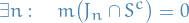
Suppose that is non-measurable subset of the real line, such as the Vitali set. Then the  measure of
  is not defined, but
and this larger set (  ) does have measure zero, i.e. it's not complete !
Motivation
Suppose we have constructed Lebesgue measure on the real line: denote this measure space by . We now wish to construct some two-dimensional Lebesgue measure on the plane  as a product measure.
Naïvely, we could take the sigma-algebra on to be  , the smallest sigma-algebra containing all measureable "rectangles"
  for
for  .
.
While this approach does define a measure space, it has a flaw: since every singleton set has one-dimensional Lebesgue measure zero,

for any subset of .
What follows is the important part!
However, suppose that is non-measureable subset of the real line, such as the Vitali set. Then the measure of is not defined (since we just supposed that is non-measurable), but
and this larger set ( ) does have measure zero, i.e. it's not complete !
Construction
Given a (possible incomplete) measure space , there is an extension  of this measure space that is complete .
The smallest such extension (i.e. the smallest sigma-algebra  ) is called the completion of the measure space.
It can be constructed as follows:
- Let
 be the set of all measure zero subsets of (intuitively, those elements of that are not already in are the ones preventing completeness from holding true)
 - Let be the sigma-algebra generated by and (i.e. the smallest sigma-algreba that contains every element of and of )
- has an extension to (which is unique if is sigma-finite), called the outer measure of , given by the infimum

Then is a complete measure space, and is the completion of .
What we're saying here is:
- For the "multi-dimensional" case we need to take into account the zero-elements in the resulting sigma-algebra due the product between the 1D zero-element and some element NOT in our original sigma-algebra
- The above point means that we do NOT necessarily get completeness, despite the sigma-algebras defined on the sets individually prior to taking the Cartesian product being complete
- To "fix" this, we construct a outer measure
 on the sigma-algebra where we have included all those zero-elements which are "missed" by the naïve approach,
Measurable functions
Let  and
and  be measurable spaces.
A function  is a measurable function if
where  denotes the preimage of the for the measurable set
  .
.
Let  .
.
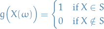
We define the indicator function of to be the function  given by
Let . Then is measurable if and only if .
Let be a measure space or a probability space.
Let  be a sequence of measurable functions.
- For each
 , the function
  is measurable
 - The function
 is measurable
 - Thus, if
 converge pointwise,
  is measurable.
Let  be a measurable space, and let
 ![$f: X \to \big[ - \infty, \infty \big]$](../../assets/latex/measure_theory_66895ba3da05558127228a3c438c5e8a19adce3c.png) .
.
The following statements are equivalent:
- is measurable.
 we have
 ![$f^{-1} \big( (c, \infty] \big) \in \mathcal{A}$](../../assets/latex/measure_theory_a1403a63281df14e6f9406be7d355f985890dd71.png) .
. we have
 ![$f^{-1} \big( [c, \infty] \big) \in \mathcal{A}$](../../assets/latex/measure_theory_7f928ebba157d8b0e32bf8ad73e9fa2873ab57d7.png) .
.![$\forall c \in (- \infty, \infty]$](../../assets/latex/measure_theory_16961a674cf394a5edb55231552df5ef2387dc61.png) we have
we have  .
.- we have
![$f^{-1} \big( [-\infty, c] \big) \in \mathcal{A}$](../../assets/latex/measure_theory_279d8a31d560b94f35569ec9df587984d4a28e58.png) .
.
A function is measurable if
![\begin{equation*}
\forall c \in [- \infty, \infty) : f^{-1} \Big( (c, \infty] \Big) \in \mathcal{A}
\end{equation*}](../../assets/latex/measure_theory_cf13df725bd4ef04ae4396b0f5bcc9e8fdddb4bf.png)
We also observe that by Proposition proposition:equivalent-statements-to-being-a-measurable-function, it's sufficient to prove
![\begin{equation*}
\forall c \in (-\infty, \infty) : f^{-1} \big( [c, \infty] \big) \in \mathcal{A}
\end{equation*}](../../assets/latex/measure_theory_8e5e1bcca38b5b97bece913a91079e5c8dbc7a7d.png)
so that's what we set out to do.
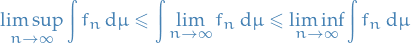
For and  , consider the following equivalent statements:
![\begin{equation*}
\begin{align*}
& & x &\in \bigg( \inf_{n \ge m} f_n \bigg)^{- 1} \Big( [c, \infty] \Big) \\
& & \inf_{n \ge m} f_n(x) &\in [c, \infty] \\
& & \inf_{n \ge m} f_n(x) &\ge c \\
&\forall n \ge m : & f_n(x) &\ge c \\
& \forall n \ge m : & x & \in f_n^{-1} \big( [c, \infty \big) \\
& & x & \in \bigcap_{n \ge m}^{\infty} f_n^{-1} \big( [c, \infty] \big)
\end{align*}
\end{equation*}](../../assets/latex/measure_theory_94af009dc1af4db3187dfbf9a593271d7e6f84f7.png)
Thus,
![\begin{equation*}
\Big( \inf_{n \ge m} f_n \Big)^{-1} \big( [c, \infty] \big) = \bigcap_{n \ge m}^{} f_n^{-1} \big( [c, \infty] \big)
\end{equation*}](../../assets/latex/measure_theory_50a948d91ff66fee7b9175dd150be89b0439004f.png)
so
![\begin{equation*}
\big( \inf_{n \ge m} f_n \big)^{-1} \big( [c, \infty] \big) \in \mathcal{A}
\end{equation*}](../../assets/latex/measure_theory_e82c9dc08e0706905a550f6f6dcfba1d845ac5bb.png)
Recall that for each , the sequence 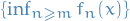 is an increasing sequence in
  . Therefore, similarily, the following are equivalent:
![\begin{equation*}
\begin{align}
& & x & \in \big( \liminf_{n \to \infty} f_n \big)^{- 1} \big( [c, \infty] \big) \\
& & \liminf_{n \to \infty} f_n(x) & \in [c, \infty] \\
& & \uparrow \lim_{m \to \infty} \inf_{n \ge m} f_n(x) &\ge c \\
& & \sup_m \inf_{n \ge m} f_n(x) &\ge c \\
& \forall N \in \mathbb{Z} : \exist m \in \mathbb{N} & \inf_{n \ge m} f_n(x) &\ge c - \frac{1}{N} \\
& \forall N \in \mathbb{N} : & x &\in \bigcup_{m \in \mathbb{N}}^{} \bigg( \inf_{n \ge m} f_n \bigg)^{-1} \bigg( \bigg[ c - \frac{1}{N}, \infty \bigg] \bigg) \\
& & x & \in \bigcap_{N \in \mathbb{N}}^{} \bigcup_{m \in \mathbb{N}}^{} \bigg( \inf_{n \ge m} f_n \bigg)^{-1} \bigg( \bigg[ c - \frac{1}{N}, \infty \bigg] \bigg)
\end{align}
\end{equation*}](../../assets/latex/measure_theory_caecf37c6ca6765e01f08e6648c9e28ae668ffe0.png)
Thus,
![\begin{equation*}
\big( \liminf f_n \big)^{-1} \big( [c, \infty] \big) = \bigcap_{N \in \mathbb{N}}^{} \bigcup_{m \in \mathbb{N}}^{} \bigg( \inf_{n \ge m} f_n \bigg)^{-1} \bigg( \bigg[ c - \frac{1}{N}, \infty \bigg] \bigg)
\end{equation*}](../../assets/latex/measure_theory_c759a8999f8697bf52bd6d4e35f493d7ca24ec11.png)
Hence,
![\begin{equation*}
\big( \liminf f_n \big)^{-1} \big( [c, \infty] \big) \in \mathcal{A}
\end{equation*}](../../assets/latex/measure_theory_e6028aa99aabfafc829083191d1bf45609989c03.png)
concluding our proof!
Basically says the same as Prop. proposition:limits-of-measurable-functions-are-measurable, but a bit more "concrete".
Let be a of subsets of a set , and let  with
with  be a sequence of measurable functions.
Furthermore, let
Then is a measurable function.
Simple functions
Let be a of subsets of a set .
A function  is called a simple function if
- it is measurable
- only takes a finite number of values
Let be a of subsets of a set .
Let ![$f : X \to [0, \infty]$](../../assets/latex/measure_theory_79e902dffac5e5c0b65197f8c0b14589c6664f65.png) be a nonnegative measurable function.
be a nonnegative measurable function.
Then there exists a sequence  of simple functions such that
 for all
 Converges to
:
Define a function  as follows. Let
and let

Then the function
obeys the required properties!
Almost everywhere and almost surely
Let be a measure or probability space.
Let  be a sequence of measurable functions
- For each the function is measurable
- The function is measurable
- Thus, if the converge pointwise, then is measurable
Let be a measure space. Let  be a condition in oe variable.
holds almost everywhere (a.e.) if

Let  be a probability space and be a condition in one variable, then holds almost surely (a.e.) if

also denoted

Let be a complete measure space.
- If is measurable and if
 a.e. then is measurable.
 - Being equal a.e. is an equivalence relation on measurable functions.
Convergence theorems for nonnegative functions
Problems
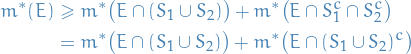
Clearly if  with
with  s.t.
s.t.  , then

hence
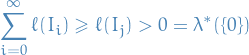
Therefore it's sufficient to prove that if  , then there exists a non-degenerate open interval
  s.t.
s.t.  . (first I said contained in , but that is a unecessarily strong statement; if contained then what we want would hold, but what we want does not imply containment).
As we know, for every there exists  such that
  and
and

Which implies
which implies

Letting  , this implies that there exists an open cover
  s.t.
s.t.
and

(this fact that this is true can be seen by considering  for all and see that this would imply
  not being a cover of , and if
  , then since
  there exists a "smaller" cover).
Thus,
Hence, letting  be s.t.

we have

as wanted!
 , we have
  for almost every
  if and only if for almost every , for all .
This is equivalent to saying
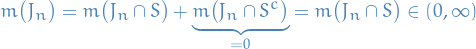
![\begin{equation*}
m \Big( f_n^{-1} \big( (-\infty, 0] \big) \Big) = 0, \quad \forall n \in \mathbb{N}
\end{equation*}](../../assets/latex/measure_theory_67584d2b69d979eee0f59c423a7e6cfbc7c4b82a.png)
if and only if
![\begin{equation*}
m \bigg( \bigcup_{n = 0}^{\infty} f_n^{-1} \Big( (-\infty, 0] \Big) \bigg) = 0
\end{equation*}](../../assets/latex/measure_theory_4acf342f12fd15b4c6d3b130fe41fb4825810116.png)
i.e.  is a set of measure zero.
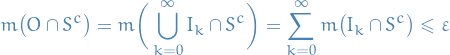
 Then clearly
![\begin{equation*}
m \bigg( \bigcup_{n=0}^{\infty} f_n^{-1} \big( (- \infty, 0] \big) \bigg) = \sum_{n=0}^{\infty} \underbrace{m \Big( f_n^{-1} \big( (- \infty, 0] \big) \Big)}_{= 0} = 0
\end{equation*}](../../assets/latex/measure_theory_b5c3b4a7db26f3d66f1400bc53d458741769e23b.png)
by the assumption.
 Follows by the same logic:
![\begin{equation*}
\sum_{n=0}^{\infty} m \Big( f_n^{-1} \big( (- \infty, 0] \big) \Big) = \underbrace{m \bigg( \bigcup_{n=0}^{\infty} f_n^{-1} \big( (- \infty, 0] \big) \bigg)}_{= 0} = 0
\end{equation*}](../../assets/latex/measure_theory_6b06dbd7651e8132421b8a66be9d25590a352936.png)
This concludes our proof.
Integration
Notation
We let
where

Stuff
Let
where  are a set of positive values.
Then the integral  of over wrt. is given by
![$f: X \to [0, \infty]$](../../assets/latex/measure_theory_975f6cbaae79dc80eb579507ef8e3c7de71d28a6.png) be a nonnegative
be a nonnegative  of
of 
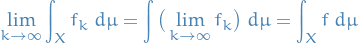
Let  be a sequence of nonnegative measurable functions on . Assume that
 for each
  for each .
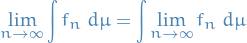
Then, we write  pointwise.
Then is measurable, and
Let  . By Proposition proposition:limit-of-measurable-functions-is-measurable, is measurable.
Since each satisfies  , we know
  .
.
- If
 , then since
  and for all we have
  , and
, and  .
.
Let  and .
and .
Step 1: Approximate by a simple function.
Let  be a simple function such that
  and
and  .
Such an exists by definition of Lebesgue integral. Thus, there are
.
Such an exists by definition of Lebesgue integral. Thus, there are  such that
  , and disjoint mesurable sets
  such that
If any  , it doesn't contribute to the integral, so we may ignore it and assume that there are no such sets.
Step 2: Find sets of large measure where the convergence is controlled.
Note that for all  we have

That is, for each and  ,
,
For and , let
And since it's easier to work with disjoint sets,
Observe that,
Then,
We don't have a "rate of convergence" on  , but on
  we know that we are
  close, and so we can "control" the convergence.
Step 3: Approximate from below.
For each if  , then let
  be such that
and otherwise, let be such that
Let  , and let
  .
.
For each  ,
,  and
and  we have
Thus,  , and
, and  ,
,
If there is a such that  , then
Otherwise (if the integral is finite), then
For every  and , there is an
  such that
For every such that
Therefore
Thus,
as wanted.
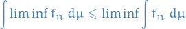
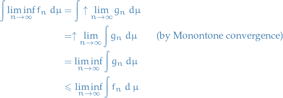
Let be any nonnegative measurable functions on .
Then
Let 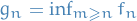 and observe
  are pointwise increasing
Properties of integrals
Let be a measure space.
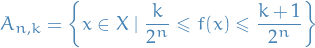
If is a nonnegative measurable function, then there is an increasing sequence of simple functions such that
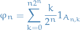
Given as above and for  , let
, let
![\begin{equation*}
\begin{split}
S_{n, k} &= f^{-1} \Big( \big[k 2^{-n}, (k + 1) 2^{-n} \big) \Big) \\
S_{n, 4^n} &= f^{-1} \Big( [2^n, \infty] \Big)
\end{split}
\end{equation*}](../../assets/latex/measure_theory_aa6b395505b8bd8701e0668288bf3f46245d7906.png)
and
Or a bit more explicit (and maybe a bit clearer),
![\begin{equation*}
f_n = \underbrace{4^n 2^{-n}}_{= 2^n} \chi_{f^{-1} \Big( [2^n, \infty] \Big)} + \sum_{k=0}^{4^n - 1} \big( k 2^{-n} \big) \chi_{f^{-1} \Big( \big[\frac{k}{2^n}, \frac{k + 1}{2^n} \big) \Big)
\end{equation*}](../../assets/latex/measure_theory_bc744558768b4a547f739ded454eaedaafbc4971.png)
For each ,  is a cover of . On each
  we have , hence on entirety of .
Consider . If  , then for
  which in turn implies
Hence  .
.
Finally, if  , then
  and for all take on values

Hence,  for all cases.
Furthermore, for any and  , there is the nesting property

so on we have  .
.
(This can be seen by observing that what we're really doing here is dividing the values takes on into a grid, and observing that if we're in then we're either in  or
or  ).
).
For  , then
so again  and is pointwise increasing.
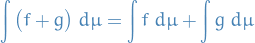
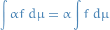
Let be a measure space.
Let
 be nonnegative, measurable functions
![$\alpha \in [0, \infty]$](../../assets/latex/measure_theory_37d5fe22c2c90662a9b0b8b33308006a3475d65c.png) s.t.
s.t.
is defined
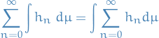
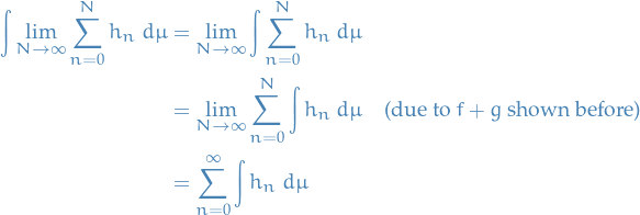
 be a sequence of nonnegative measurable functions.
Then
Finite sum
Scalar multiplication
Infinte sums
Let and be increasing sequence of simple functions converging to , , respectively.
Note  is aslo increasing to
  .
.
By monotone convergence theorem
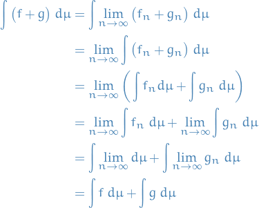
The argument is similar for products.
Finally, 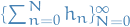 is an increasing sequence of nonnegative measurable functions, since sums of measurable functions is a measurable function.
Thus, by monotone convergence and the result for finite sums
Integrals on sets
Let be a measure or probability space.
If  is a sequence of disjoint measurable sets then
Let be a measure or probability space.
If is a simple function and is a measurable set, then  is a simple function.
Let be a measure or probability space.
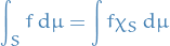
Let be a nonnegative measurable function and .
The integral of on is defined to be
Let be a measure or probability space.
Let be a nonnegative measurable function.
If
and are disjoint measurable sets, then
If
are disjoint measurable sets, then
Let be a measure or probability space.
If is a nonnegative measurable function, then ![$\mu_f: \mathcal{A} \to [0, \infty]$](../../assets/latex/measure_theory_5431344eb18be9cd48ff98f38d15812bb8f3f3a3.png) defined by
defined by  :
:
is a measure on .
If  , then
 ![$P_f: \mathcal{A} \to [0, \infty]$](../../assets/latex/measure_theory_595ab36a9344eed11eb64916b5fa997660643f02.png) defined by :
defined by :
The (real) Gaussian measure on is defined as:
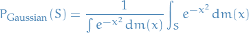
where denotes the Lebesgue measure.
A Gaussian probability measure can also be defined for an arbitrary Banach space as follows:
Then, we say is a Gaussian probability measure on if and only if is a Borel measure, i.e.
such that  is a real Gaussian probability measure on for every linear functional
  , i.e.
  .
.
Here we have used the notation  , defined
where  denotes the Borel measures on .
Integrals of general functions
Let be a measure or probability space.
If ![$f: \Omega \to [- \infty, \infty]$](../../assets/latex/measure_theory_27db8ee19d1a570b0cf117dd687777fac66160ec.png) is a measurable function, then the positive and negative parts are defined by
is a measurable function, then the positive and negative parts are defined by
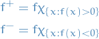
Note:  and
and  are nonnegative.
Let be a measure or probability space.
If is a measurable function, then and  are measurable functions.
Let be a measure or probability space.
- A nonnegative function is defined to be integrable if it is measurable and
 .
. - A function is defined to be integrable if it is measurable and
 is integrable.
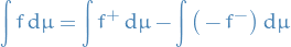
For an integrable function , the integral of is defined to be
On a set , the integral is defined to be
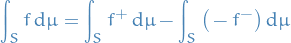
Note that , but in the actual definition of the integral, we use  .
.
Let be a measure or probability space.
If and are real-valued integrable functions and , then
(Scalar multiplication)
(Additive)
Let be a measure or probability space.
Let and be measurable functions s.t.

If is integrable then is integrable.
Examples
Consider with Lebesgue measure. Is  integrable?

And
and
therefore
Thus, is integrable.
Lebesge dominated convergence theorem
Let be a measure or probability space.
Let be a nonnegative integrable function and let  be a sequence of (not necessarily nonnegative!) measurable functions.
Asssume and all are real-valued.
If and such that
and the pointwise limit

exists.
Then
That is, if there exists a "dominating function"  , then we can "move" the limit into the integral.
Since and such that  , we find that
  and
and  are nonnegative.
Consider 
From Fatou's lemma, we have
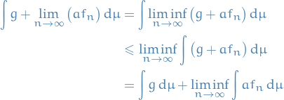
Therefore
Consider  , then
(this looks very much like Fatou's lemma, but it ain't; does not necessarily have to be nonnegative as in Fatou's lemma)
Consider 

Therefore,
Which implies
Since  , we then have
  exists and is equal to
 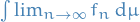 .
.
Examples of failure of dominated convergence
Where dominated convergence does not work
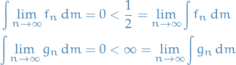
On with Lebesgue measure, consider
![\begin{equation*}
\begin{split}
f_n &= \chi_{[n, n + \frac{1}{2}]} \\
g_n &= \arctan \big( x - n \big) + \frac{\pi}{2}
\end{split}
\end{equation*}](../../assets/latex/measure_theory_86b9124678b092e327558bdc249245b93ada07c3.png)
such that ![$g_n \in [0, \pi]$](../../assets/latex/measure_theory_1cda4a0be5367504c88a0871f4e46c2cc110f596.png) instead of
instead of ![$[- \frac{\pi}{2}, \frac{\pi}{2}]$](../../assets/latex/measure_theory_4c0845ce4ba68814a80ace45d8f5f56fddfec79f.png) as "usual" with
as "usual" with  .
.
Both of these are nonnegative sequences that converge to  pointwise.
Notice there is no integrable dominating function for either of these sequences:
- would require a dominating function to have infinite integral, therefore no dominating integrable function exists.
 on the right, and so a dominating function would have to be above
  on some interval
  which would lead to infinite integral.
Thus, Lebesgue dominated convergence does not apply
Noncummtative limits: simple case

Noncommutative limits: another one
Consider with Lebesgue measure and
![\begin{equation*}
f(x) = \frac{1}{x} \chi_{[1, \infty)} - \frac{1}{\left| x \right|} \chi_{(-\infty, -1]}
\end{equation*}](../../assets/latex/measure_theory_14635fa0f57a58ce700b3856836b8bcda95d51e0.png)
Consider  and $ b > 1$ and
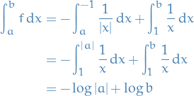
Note that  , so is not integrable.
Consider
![\begin{equation*}
\begin{split}
\lim_{N \to \infty} \int \chi_{[-N, N]} f \dd{x} &= \lim_{N \to \infty} \Big( - \log \left| - N \right| + \log N \Big) = \lim_{N \to \infty} 0 = 0 \\
\lim_{N \to \infty} \int \chi_{[-N, 2N]} f \dd{x} &= \lim_{N \to \infty} \Big( - \log N + \log 2N \Big) = \lim_{N \to \infty} \log 2 = \log 2
\end{split}
\end{equation*}](../../assets/latex/measure_theory_7503b43d535ab9bfd060eaa19b94e17bd2de244e.png)
Commutative limits
Consider
![\begin{equation*}
\lim_{N \to \infty} \lim_{M \to \infty} \int \chi_{[-M, N]} f \dd{x} = \lim_{M \to \infty} \lim_{N \to \infty} \int \chi_{[- M, N]} f \dd{x}
\end{equation*}](../../assets/latex/measure_theory_1591ddcfb29c1faa905731373db01dfdb888bb3e.png)
We know that  is integrable and for all
  and ,
and ,
By multiple applications of LDCT
![\begin{equation*}
\begin{split}
\lim_{N \to \infty} \lim_{M \to \infty \to \infty} \int \chi_{[-M, N]} f \dd{x} &= \lim_{N \to \infty} \int \chi_{(-\infty, N]} f \dd{x} \\
&= \int \chi_{(-\infty, \infty)} f \dd{x} \\
&= \int f \dd{x} \\
&= \int \chi_{(-\infty, \infty)} f \dd{x} \\
&= \lim_{M \to \infty} \int \chi_{[-M, \infty)} f \dd{x} \\
&= \lim_{M \to \infty} \lim_{N \to \infty} \int \chi_{[-M, N]} f \dd{x}
\end{split}
\end{equation*}](../../assets/latex/measure_theory_dbd2a8cecbc43b92c2b5adc3837df5b30a770f80.png)
Showing that in this case the limits do in fact commute.
Riemann integrable functions are measurable
All Riemann integrable functions are measurable.
For any Riemann integrable function, the Riemann integral and the Lebesgue integral are equal.
Almost everywhere and Lp spaces
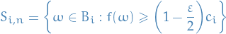
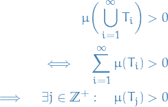
If is a nonnegative, measurable function, and  , then
  .
.
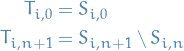
For  , let
, let
![\begin{equation*}
\begin{split}
T_0 &= f^{-1} \Big( (1, \infty] \Big) \\
T_n &= f^{-1} \bigg( \bigg( \frac{1}{n + 1}, \frac{1}{n} \bigg] \bigg), \quad n \in \mathbb{Z}^+
\end{split}
\end{equation*}](../../assets/latex/measure_theory_2ceab74592bc736a2823d5c8f0aa92dafd661f57.png)
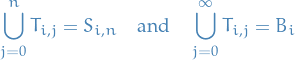
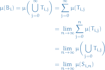
Observe the  are disjoint and
![\begin{equation*}
\bigcup_{i = 1}^{\infty} T_i = f^{-1} \bigg( (0, \infty] \bigg)
\end{equation*}](../../assets/latex/measure_theory_93b55f6349b02c3782503473a25b3f7b47350719.png)
Suppose that  . This implies that
  on a set of positive measure, i.e.
![\begin{equation*}
\mu \bigg( f^{-1} \Big( (0, \infty] \Big) \bigg) > 0
\end{equation*}](../../assets/latex/measure_theory_e85507015506242700deeda1834343a94f438944.png)
but this implies that
Thus,
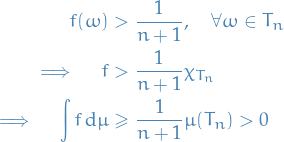
which is a contradiction, hence .
Let and be integrable.
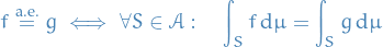
 is the set of all equivalence classes of integrable functions wrt. the equivalence relation given by a.e. equality, i.e.

If is an integrable function, the  norm is
If ![$[f] \in L^1(\dd{\mu})$](../../assets/latex/measure_theory_febf1d9c9d9fc46e4fc2d9e79dd425642660a25e.png) and
and ![$g \in [f]$](../../assets/latex/measure_theory_0674799b02ef974d9bce66406bc2481c9c7bb951.png) , the integral and norm are defined to be
, the integral and norm are defined to be
![\begin{equation*}
\begin{split}
\int [f] \dd{\mu} &= \int g \dd{\mu} \\
\norm{[f]}_{L^1} &= \norm{g}_{L^1}
\end{split}
\end{equation*}](../../assets/latex/measure_theory_6917d223cd066748131b36bb5557b619ee598345.png)
If ![$[f], [g], [h] \in L^1$](../../assets/latex/measure_theory_e32b14a7500cc43f20c1a1657905bfee0ed6d43e.png) , then
, then ![$[f + g] \in L^1$](../../assets/latex/measure_theory_9ee9da136403a0f769d8056adb9124c5934f6f3f.png) , and
, and
![\begin{equation*}
\norm{[f - g]}_{L^1} \le \norm{f - g}_{L^1} + \norm{[h - g]}_{L^1}
\end{equation*}](../../assets/latex/measure_theory_280aa5fd4f0f61951e29cf2fba4c67eb4af32159.png)
is a real vector space with addition and scalar multiplication given pointwise almost everywhere.
Functions taking on  on a set of zero measure are fine!
These functions are still the almost everywhere equal to some integrable function (even those these infinite-valued functions are integrable), hence these are in .
![\begin{equation*}
d \big( [f], [g] \big) = \norm{[f - g]}_{L^1}
\end{equation*}](../../assets/latex/measure_theory_a16835d39d8c52702508e6531de8f45a43dbceb7.png)
Let ![$\left\{ [f_k] \right\}$](../../assets/latex/measure_theory_adf0c6a74e755c8ef23b722bb511497982e81a93.png) be a Cauchy sequence. Since the
be a Cauchy sequence. Since the  are integrable, we may assume we choose valued representatives.
For , let  be such that for
  ,
,
and  .
.
Thus,
and
Thus,  is finite almost everywhere. Thus, this series is infinite on a set of measure zero, so we may assume the representatives are zero there and the sum is finite at each .
Thus,  converges everywhere.
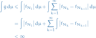
Let
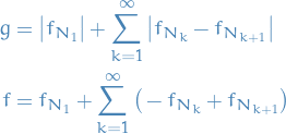
(observe that the last part is just rewriting the  ).
).
By monotone convergence theorem
Observe that pointwise
Applications to Probability
Notation
- is a probability space
- Random variable is a measurable function
 denotes the Borel sigma-algebra on
  denotes the probability distribution measure for
  be a sequence of random events
 be a sequence of finitely many random events
Probability and cumulative distributions
An elementary event is an element of .
A random event is an element of
A random variable is a measurable function from to ![$\Big( [- \infty, \infty], \mathcal{B} \big( [- \infty, \infty] \big) \Big)$](../../assets/latex/measure_theory_71661c6fca4577bd7a8dc72d729db6c0c7455aef.png) .
.
Let
 be a measure space and
  be a measurable space
- be a measurable function
Then we say that the push-forward of by is defined

The probability distribution measure of , denoted ![$\rho_X: \mathcal{B}(\mathbb{R}) \to [0, 1]$](../../assets/latex/measure_theory_a5c7220fd4e2a7451ed9120399b51f8339ac82f6.png) , is defined
, is defined

Equivalently, it's the push-forward of  by :
by :
In certain circles not including measure-theorists (existence of such circles is trivial), you might hear talks about "probability distributions". Usually what is meant by this is for some random variable .
That is, a "distribution of " usually means that there is some probability space in which is a random variable, i.e. and the "distribution of " is the corresponding probability distribution measure!
Confusingly enough, they will often talk about " distribution of ", in which case is NOT a probability measure, but denotes a probability distribution measure of the random variable.
The cumulative distribution function of , denoted ![$F_X: \mathbb{R} \to [0, 1]$](../../assets/latex/measure_theory_857de4732cc5895e72b48743bb1ed0b6c6ef9120.png) , is defined by
, is defined by
![\begin{equation*}
\forall x \in \mathbb{R}, \quad F_X(x) = P(X \le x) = \rho_X \big( (- \infty, x] \big)
\end{equation*}](../../assets/latex/measure_theory_1135df16d8d98e78eda428fdded8af11029fc26f.png)
where is the probability distribution measure of .
The probability distribution measure is a probability measure on the Borel sets  .
.

If  is a disjoint sequence of sets in
  , then
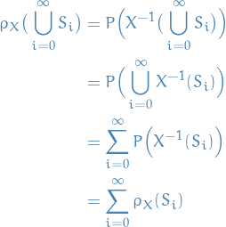
so satisfies countable additivity and is a measure.
Finally,

so is a probability measure.
 is increasing
 and
and 
- is right continuous (i.e. continuous from the right)

If
 , then
![\begin{equation*}
\begin{split}
F_X(x) &= P(X \le x) \\
&= P \Big( X^{-1} \big( (- \infty, x] \big) \Big) \\
& \le P \Big( X^{-1} \big( ( -\infty, x] \big) \Big) + P \Big( X^{-1} \big( (x, y] \big) \Big) \\
&= P \Big( X^{-1} \big( (-\infty, x] \cup (x, y] \big) \Big) \\
&= P \Big( X^{-1} \big( (- \infty, y] \big) \Big) \\
&= F_X(y)
\end{split}
\end{equation*}](../../assets/latex/measure_theory_02e5898fb6b34b5dbd3e516b4c58fb5d27ddfe1b.png)
Consider the limit as
 . Let
. Let
![\begin{equation*}
\begin{split}
T_0 &= X^{-1} \big( (- \infty, 0] \big) \\
T_n &= X^{-1} \big( (n - 1, n] \big), \quad \forall n \in \mathbb{Z}^+
\end{split}
\end{equation*}](../../assets/latex/measure_theory_822502b5a0806137387a045422e41a8d00ed4b6e.png)
so
Then,
![\begin{equation*}
\begin{split}
1 &= P (\Omega) = P \bigg( \bigcup_{i=0}^{\infty} T_i \bigg) \\
&= \lim_{n \to infty} \sum_{i=0}^{n} P(S_i) \\
&= \lim_{n \to \infty} \bigg( P \Big( X^{-1} \big( (- \infty, 0] \big) \Big) \bigg) + \sum_{i=1}^{n} P \bigg( X^{-1} \Big( (n - 1, n] \Big) \bigg) \\
&= \lim_{n \to \infty} P \bigg( X^{-1} \Big( (- \infty, n] \Big) \bigg) \\
&= \lim_{n \to \infty} F_X(n)
\end{split}
\end{equation*}](../../assets/latex/measure_theory_c85daac3994fefdf28c3cd1e69dd2a502d02db52.png)
which, since
is increasing implies
Let
 and . Let
![\begin{equation*}
S_n = \bigg( x, x + \frac{1}{n} \bigg]
\end{equation*}](../../assets/latex/measure_theory_71877cd7b7156217e1f928f060006ff74416c33a.png)
The
 are nested, and similarily
  are nested.
![\begin{equation*}
\begin{split}
0 &= P (\emptyset) = P \bigg( x^{-1} \bigg( \bigcup_{i=0}^{\infty} S_i \bigg) \bigg) \\
&= \lim_{n \to \infty} P \Big( X^{-1}(S_n) \Big) \\
&= \lim_{n \to \infty} P \bigg( X^{-1} \bigg( \bigg(x, x + \frac{1}{n} \bigg] \bigg) \bigg) \\
&= \lim_{n \to \infty} P \bigg( X^{-1} \bigg( \bigg( - \infty, x + \frac{1}{n} \bigg] \bigg) \bigg) - P \bigg( X^{-1} \bigg( \bigg(-\infty, x \bigg] \bigg) \bigg) \\
&= \lim_{n \to \infty} \bigg[ F_X \bigg( x + \frac{1}{n} \bigg) - F_X(x) \bigg]
\end{split}
\end{equation*}](../../assets/latex/measure_theory_3f72b108040e545c8a2dbe673817e5955c4dd7a7.png)
Thus, given
, there exists such that
Let
 so
so
Radon-Nikodym derivatives and expectations
Let
- be a rv.
- its probability distribution measure
- its cumulative distribution function
- a Borel measureable function
The following are equivalent:

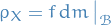
- is a Radon-Nikodym derivative for wrt.
 (the Lebesgue measure but restricted to Borel measurable sets)
(2) and (3) are immediately equivalent:
![\begin{equation*}
\rho_X \Big( (- \infty, x] \Big) = F_X(x) = \int_{-\infty}^{x} f(s) \dd{s} = \int_{-\infty}^{x} f \dd{m}
\end{equation*}](../../assets/latex/measure_theory_6826f1b8d841609a361882c3b6b70bc5ea1174ef.png)
iff (2) or (3) holds when considering only sets of the form ![$(- \infty, x]$](../../assets/latex/measure_theory_e122470acfe9dda86dc876d6b068fadc47cc17be.png) .
.
This statement is also equivalent to (1).
Thus (1) is equivalent to (2) or (3) restricted to sets of the form ![$(-\infty, x]$](../../assets/latex/measure_theory_4da7df6ea37290e01a6b13bd339c125dc9d812cd.png) .
.
However, sets of the form generate , so from the Carathéodory extension theorem this gives  .
.
To prove  more rigorously, let
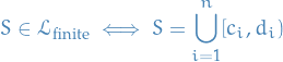
for ![$c_i, d_i \in [-\infty, \infty]$](../../assets/latex/measure_theory_879949f8d7167858f9f8cf9fe0fb70cc850702cf.png) s.t.
s.t.  and none of these intervals overlap. That is all finite unions of left-closed, right-open, disjoint intervals.
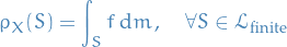
Also let
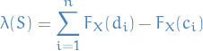
Observe that
![\begin{equation*}
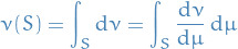
\lambda(S) = \sum_{i=1}^{n} \bigg[ \int_{-\infty}^{d_i} f(x) \dd{x} - \int_{-\infty}^{c_i} f(x) \dd{x} \bigg] = \sum_{i=1}^{n} \int_{c_i}^{d_i} f(x) \dd{x} = \int_S f \dd{m}
\end{equation*}](../../assets/latex/measure_theory_a1afc8f6f2c8e420ab88be7447f2e38b913fb942.png)
and that
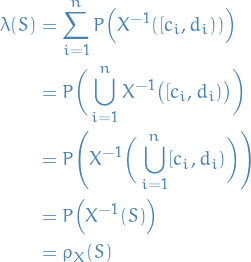
One can show that  is a premeasure space. Therefore, by the Carathéodory extension theorem, there is a measure on s.t.

Furthermore, since  , is unique! But both the measures
  and
and  satisfy these properties, thus
which is the definition of being a Radon-Nikodym derivative of wrt. Lebesgue measure restricted to the Borel σ-algebra, as wanted.
A function is a probability density function for if is a Radon-Nikodym derivative of the probability distribution measure , wrt. Lebesgue measure restricted to Borel sets, i.e.
Expectation via distributions
Expectation of a random variable is
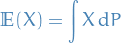
If  is a nonnegative function that is measurable, then
![\begin{equation*}
\mathbb{E} \big[ g(X) \big] = \int g(s) \dd{\rho_X(s)}
\end{equation*}](../../assets/latex/measure_theory_58b872956e73f042002d8b23eb8c33aa0d3cde55.png)
If is the characterstic function, then, if  ,
,
so

Multiplying by constants and summing over different characteristic functions, we get the result to be true for any simple function.
Given a nonnegative function , let  be an increasing sequence of simple functions converging pointwise to .
Note  is the increasing limit of
  . By two applications of Monotone Convergence
![\begin{equation*}
\begin{split}
\mathbb{E} \big[ g(X) \big] &= \int g(X) \dd{P}\\
&= \int \lim_{n \to \infty} g_n(X) \dd{P} \quad\\
&= \lim_{n \to \infty} \int g_n(X) \dd{P} \quad \text{(by MC)} \\
&= \lim_{n \to \infty} \int g_n \dd{\rho_X} \quad \text{(by above)}\\
&= \int g \dd{\rho_X} \quad \text{(by MC)}
\end{split}
\end{equation*}](../../assets/latex/measure_theory_011ad9343b3c73146cd5357e27623d0048277ef0.png)
This techinque, of going from characterstic function → simple functions → general functions, is used heavily, not just in probability theory.
Independent events & Borel-Cantelli theorem
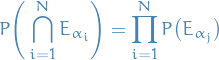
A collection of random events  are independent events if for every finite collection of distinct indices
  ,
,
A random event  occurs at if
  .
.
The probability that the event occurs is  .
.
If  are independent then
  are also independent.
Prove that  are independent.
Consider  , we want to prove
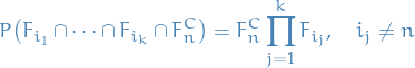
RHS can be written
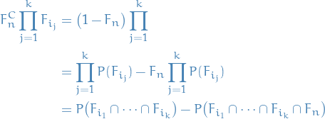
which is equal to LHS above, and implies that the complement is indeed independent.
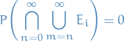
The condition that infinitively many of the events occurs at  is
is
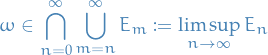
This is equivalent to

where we have converted the  and
and  .
.
Furthermore,  is itself a random event.
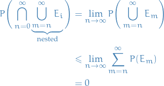
If
 then probability of infinitely many of the events occuring is 0, i.e.
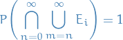
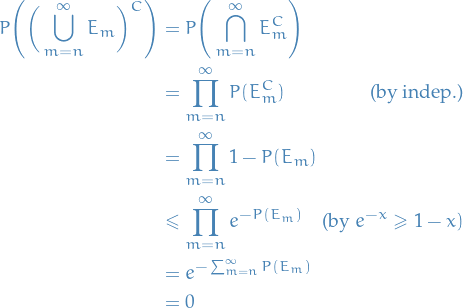
If the
are independent and  , then probability of infinitely many of the events occuring is 1, i.e.
Suppose
 .
.
Suppose
are now independent and that .
Fix . Then
Chebyshev's inequality
Let be a probability space.
If is a random variable with mean and variance  , then
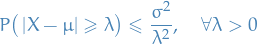
Let

Then  everywhere, so
![\begin{equation*}
\sigma^2 = \mathbb{E} \big[ \big( X - \mu \big)^2 \big] \ge \lambda^2 \mathbb{E} \big[ \chi_E \big] = \lambda^2 P(E)
\end{equation*}](../../assets/latex/measure_theory_afe5a26fe68a2dc369c6842791542f5d9f5bcae3.png)
Hence,

Independent random variables
Let
- be a probability space.
A collection of σ-algebras  , where
  for all , is independent if for every collection of events
  s.t
s.t  for all , then is a set of independent events.
A collection of random variables  is independent if the collection of σ-algebras they generate is independent.
A sequence of random variables  is independent and identically distributed (i.i.d) if they are independent variables and for
  we have

where  is the cumulative distribution function for
  .
.
Let and  be independent.
- We have
- If
![$\mathbb{E} \big[ \left| X \right| \big] = 0$](../../assets/latex/measure_theory_f4839615bca9740a070cd50282abcd49b624299c.png) or
or ![$\mathbb{E} \big[ \left| Y \right| \big] = 0$](../../assets/latex/measure_theory_9c2a3e0176324c0303d6e99d95778d8ad8444e90.png) then
then ![$\mathbb{E} \big[ \left| XY \right| \big] = 0$](../../assets/latex/measure_theory_761e7445761b7eb7decf7480a3f579dde5590770.png)
If
![$\mathbb{E} \big[ \left| X \right| \big] > 0$](../../assets/latex/measure_theory_cbb7cd0c3b3a0b7ec2194b26ea2f9c64511309c2.png) and
and ![$\mathbb{E} \big[ \left| Y \right| \big] > 0$](../../assets/latex/measure_theory_d49dbff5ad4b491ca50fc08dbce0112bd500a9ae.png) , then
, then
![\begin{equation*}
\mathbb{E} \big[ \left| XY \right| \big] = \mathbb{E} \big[ \left| X \right| \big] \mathbb{E} \big[ \left| Y \right| \big]
\end{equation*}](../../assets/latex/measure_theory_8da658297f17540bbbc9cb6726bb1d2bbebbc692.png)
- If
Furthermore, if
![$\mathbb{E} \big[ \left| X \right| \big] < \infty$](../../assets/latex/measure_theory_a7ed308ceeb09933497e2a2acc8b07d915339ef8.png) and
and ![$\mathbb{E} \big[ \left| Y \right| \big] < \infty$](../../assets/latex/measure_theory_10ed410a5b735e421f331da4aa674c32c022cda7.png) , then
, then
![\begin{equation*}
\mathbb{E} \big[ XY \big] = \mathbb{E} \big[ X \big] \mathbb{E} \big[ Y \big]
\end{equation*}](../../assets/latex/measure_theory_127c9fbe3926cc0ee673512d405f56dccef62e67.png)
Consider
- first nonnegative functions
- subcase
![$\mathbb{E} \big[ X \big] = 0$](../../assets/latex/measure_theory_384ab7ec94ace068cc33f7a3b4036e557945d4e1.png)
Since is nonnegative
![\begin{equation*}
0 = \mathbb{E} \big[ X \big] = \int X \dd{P} \implies X \overset{\text{a.s.}}{=} 0
\end{equation*}](../../assets/latex/measure_theory_3adfb341d10c51cb63db312ac51f907340ca7087.png)
Thus,  so
so ![$\mathbb{E} \big[ XY \big] = 0$](../../assets/latex/measure_theory_ef0626a72b6e48ffbef4e690927fe3ebe3289d4d.png) .
.
Now consider the subcase where ![$\mathbb{E} \big[ X \big] > 0$](../../assets/latex/measure_theory_10c6cdf7c0ab3ad30df17078595f922f9f87633c.png) and
and ![$\mathbb{E} \big[ Y \big] > 0$](../../assets/latex/measure_theory_c59194d819989aa539ba17b5ee03462e949ce8fe.png) .
.
Let  and
and  be the σ-algebras generated by and .
Observe that  and
and  are measure spaces. Let be an increasing sequence of simple functions that are measurable wrt. and similarily
  simple increasing to and measurable.
As simple functions, these can be written as
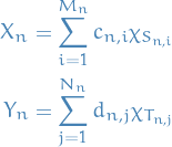
Then,
![\begin{equation*}
\begin{split}
\mathbb{E} \big[ X_n Y_n \big] &= \int \sum_{i=1}^{M_n} \sum_{j=1}^{N_n} c_{n, i} d_{n, j} \chi_{S_{n, i}} \chi_{T_{n, j}} \dd{P} \\
&= \sum_{i=1}^{M_n} \sum_{j=1}^{N_n} c_{n, i} d_{n, j} P \Big( S_{n, i} \cap T_{n, j} \Big) \\
&= \sum_{i=1}^{M_n} \sum_{j=1}^{N_n} c_{n, i} d_{n, j} P \big( S_{n, i} \big) P \big( T_{n, j} \big) \\
&= \bigg( \sum_{i=1}^{M_n} c_{n, i} P \big( S_{n, i} \big) \bigg) \bigg( \sum_{j=1}^{N_n} d_{n, j} P\big(T_{n, j} \big) \bigg) \\
&= \mathbb{E} \big[ X_n \big] \mathbb{E} \big[ Y_n \big]
\end{split}
\end{equation*}](../../assets/latex/measure_theory_a8103249f0b23d4dc0542716a5f5c9d173d60a25.png)
Since  increases to
  , by MCT
Dividing into positive & negative parts & summing gives  .
.
Strong Law of Large numbers
Notation
 are i.i.d. random variables, and we will assume
![\begin{equation*}
\mathbb{E}[X_i] < \infty \quad \text{and} \quad \text{Var}(X_i) < \infty
\end{equation*}](../../assets/latex/measure_theory_ce80998071f168839f18af296b335d9ed4193f3a.png)
Stuff
Let be a probability space and be a sequence of i.i.d. random variables with
![\begin{equation*}
\mu := \mathbb{E}[X_i] < \infty \quad \text{and} \quad \sigma^2 := \text{Var}(X_i) < \infty
\end{equation*}](../../assets/latex/measure_theory_b5a2be16754e0eac4426741ec560e711c0165643.png)
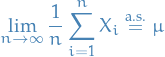
Then the sequence of random variables  converges almost surely to , i.e.
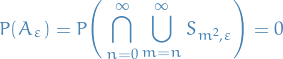
This is equivalent to  occuring with probability 0, and this is the approach we will take.
First consider  .
.
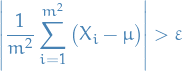
For and , let
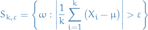
and
Since  are i.i.d. we have
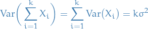
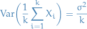
and since variance rescales quadratically,
Using Chebyshev's inequality
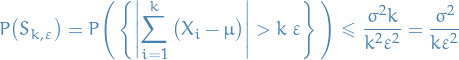
Observe then that with  , we have
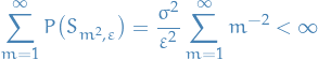
And so by Borel-Cantelli, since this is a sequence of independent random variables, we have
In particular, for any , there are almost surely only finitely many with
Step: showing that we can do this for any .
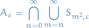
Consider  . Observe that by countable subadditivity,
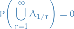
Now let  , which occurs almost surely from the above. For any , let
Since , there are only finitely many s.t.
as found earlier (the parenthesis are indeed different here, compared to before). Therefore
is arbitrary, so this is true for all . Hence,
This proves that there is a subsequential limit almost surely.
Step: subsequential limit to "sequential" limit.
Given , let be such that  . Since are nonnegative
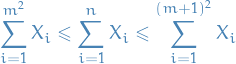
and therefore
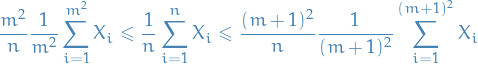
and since ,
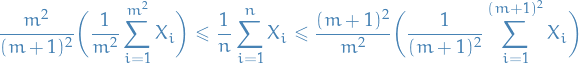
Since the first and the last expressions converge to ,t by the squeeze theorem we have
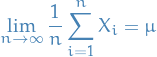
Step: Relaxing nonnegativity assumption on .
Suppose is not necessarily nonnegative. Since, by assumption, has finite expectation, is integrable. Therefore we know that the positive and negative parts of , denoted  , are also integrable. Therefore we can compute the expectations
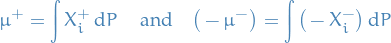
Similarily, we have that the variance of is finite, which allows us to the apply the result we found for being nonnegative to both  and
and  :
:
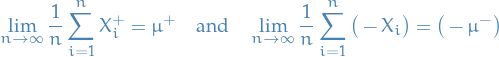
Let  be the set where the mean of the positive / negative part converges. Since
(since otherwise the limit would not converge almost surely). We then have
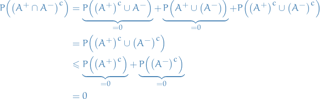
Thus, almost surely,  , and on this we have convergence, so
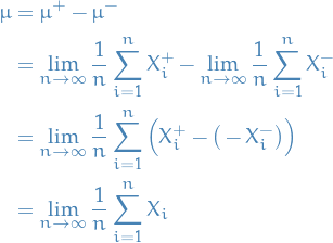
Concluding our proof.
Ergodic Theory
Let be a measure-preserving transformation on a measure space with  , i.e. it's a probability space.
Then is ergodic if for every  we have

Bochner integrable
The Bochner integral is a notion of integrability on Banach spaces, and is defined in very much the same way as integrability wrt. Lebesgue-measure.
Let be a measure space and  a Banach space.
A simple function is defined similarily as before, but now taking values on a Banach space instead. That is,
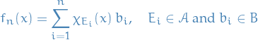
with the integral
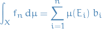
A measurable function  is said to be Bochner integrable if there exists a sequence of integrable simple functions such that
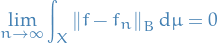
where the integral on the LHS is an ordinary Lebesgue integral.
If this is the case, then the Bochner integral is defined
It can indeed be shown that a function is Bochner integrable if and only if  , the Bochner space, defined similarily as L1-space for functions but with the absolute value replaced by the
  .
.
Concentration inequalities
Stochastic processes
Let
 be a filtration
 be an
be an  martingale
 be an
be an  stopping time
such that one of the following holds:
 such that
![$\mathbb{E}[\tau] < \infty$](../../assets/latex/measure_theory_8df09c95f86cc43dc18e05643b092bcf5c0ed750.png) and there exists a constatn
and there exists a constatn  s.t. for all
  ,
,
![\begin{equation*}
\mathbb{E} \big[ \left| X_{t + 1} - X_t \right| \mid \mathcal{F}_t \big] \le c
\end{equation*}](../../assets/latex/measure_theory_f5e02bae54ba58678204010c90aae14d2be4ffb5.png)
almost surely on the even that
 .
.
 such that
  almost surely for all
Then  is a.s. well-defined and
 ![$\mathbb{E}[X_{\tau}] = \mathbb{E}[X_0]$](../../assets/latex/measure_theory_82948a934352eea2952f8bfe47753bc0c9a3f810.png) .
.
Furthermore, when  is supersub-martingale rather than a martingale, then equality is replaced with lessgreather-than, respectively.
Let  be a supermartingale with
  a.s. for all .
Then for any
![\begin{equation*}
\mathbb{P} \bigg( \sup_{t \in \mathbb{N}} X_t \ge \varepsilon \bigg) \le \frac{\mathbb{E}[X_0]}{\varepsilon}
\end{equation*}](../../assets/latex/measure_theory_84492b275ebda66c6570d1bd84ca669f463b7733.png)
Let  be the event that
  and
and  , where we assume
  so that
  if
if  for all
  .
.
Clearly is a stopping time and  . Then by Doob's optional stopping theorem and an elementary calculation
![\begin{equation*}
\begin{split}
\mathbb{E} [X_0] & \ge \mathbb{E}[X_{\tau}] \\
&\ge \mathbb{E} \big[ X_{\tau} \1 \left\{ \tau \le n \right\} \big] \\
&\ge \mathbb{E} \big[ \varepsilon \1 \left\{ \tau \le n \right\} \big] \\
&= \varepsilon \mathbb{P} (\tau \le n) = \varepsilon \mathbb{P} (A_n)
\end{split}
\end{equation*}](../../assets/latex/measure_theory_94b8b81bf7fe44c285cfefc52fe78eb1118bd0f2.png)
Course: Advanced Probability
Notation
 is used as a binary operation which takes minimum of the two arguments
 is used as a binary operation which takes maxmium of the two arguments
Lecture 1
Notation
 denotes a measurable space (with a measure it becomes a measure space)
 denotes the set of measurable functions wrt.

and non-negative measurable functions
![\begin{equation*}
m \mathcal{E}^{ + } := \left\{ f: E \to [0, \infty], f \text{ measurable wrt. } \mathcal{B}(\mathbb{R}) \right\}
\end{equation*}](../../assets/latex/measure_theory_e754d49931a63df28e637dfcfb5d3a5e0caebcb5.png)
We write
Stuff
Let  be a measure space.
Then there exists a unique ![$\tilde{\mu}: m \mathcal{E}^{ + } \to [0, \infty]$](../../assets/latex/measure_theory_b2e4fdbc02f89d88c2fc919c414c6e74699f8a39.png) s.t.
s.t.
 for all
Linearity

for all
 with
with  .
.
-
for
 pointwise.
 and
and  be finite or
 .
.
There exists a unique measure  on
on  called the product measure

Let  . For
. For  define
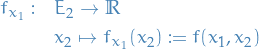
Then  is
is 
 . Hence, we can define
Then  is
is  and
and
where is the product measure.
Applying the above in both directions, we have

with

and
Conclusion:

Lecture 2: conditional expectation
Notation
 a probability space, i.e.
- denotes rv, i.e. is
 and integrable, with expectation
![\begin{equation*}
\mathbb{E} \big[ X \big] = \int X \dd{\mathbb{P}}
\end{equation*}](../../assets/latex/measure_theory_fb7b4bd20f047add86c081e6fac8f3cccaf18f89.png)
Also write
![\begin{equation*}
\mathbb{E} \big[ X 1_A \big] = \int_A X \dd{\mathbb{P}}, \quad \forall A \in \mathcal{F}
\end{equation*}](../../assets/latex/measure_theory_96acdb1cce8a64aebc57cb78f7401b63d20fe140.png)
or, as we're used to,
 instead of
Stuff
Let  with
with  .
.
Then
is called the conditional probability of given .
Similarily, we define
![\begin{equation*}
\mathbb{E} \big[ X \mid B \big] = \frac{\mathbb{E}[X 1_B]}{\mathbb{P}(B)}
\end{equation*}](../../assets/latex/measure_theory_1e9e33511ea4e04d0d2b93b6e59baf140240ac27.png)
to be the conditional expectation of given .
- Quite restrictive since we require probability of to be non-zero
- Goal: improve prediction for if additional "information" is available
- "Information" is modelled by a sigma-algebra

- "Information" is modelled by a sigma-algebra
Let  be a sequence of disjoint events, whose union is . Set
For any integrable random variable , we can define
![\begin{equation*}
Y = \sum_{n \in \mathbb{N}}^{} \mathbb{E} \big[ X \mid B_n \big] 1_{B_n}
\end{equation*}](../../assets/latex/measure_theory_df0b9f2767d97d3a5e3b87e10ea91d7c6a6b2dfa.png)
where we set
![\begin{equation*}
\mathbb{E} \big[ X \mid B_n \big] =
\begin{cases}
\frac{\mathbb{E} [ X 1_{B_n}]}{\mathbb{P}(B_n)} & \text{if } \mathbb{P}(B_n) > 0 \\
0 & \text{if } \mathbb{P}(B_n) = 0
\end{cases}
\end{equation*}](../../assets/latex/measure_theory_cb9ab6ebd3778592daaf856ee81c1ce9ae052dd8.png)
Notice that
- in (discrete) definition of conditional expectation is
![\begin{equation*}
Y(\omega) = \sum_{n \in \mathbb{N}}^{} \mathbb{E} \big[ X \mid B_n \big] 1_{B_n}(\omega)
\end{equation*}](../../assets/latex/measure_theory_de58a386a26a73adfa6a4af4e31476f647bd063e.png)
Let
![$A \in \mathcal{B}([-\infty, \infty])$](../../assets/latex/measure_theory_80ea66eaeaaf042e5dc2c64f20a6b901294f66b1.png) , then
, then
![\begin{equation*}
\begin{split}
Y^{-1}(A) &= \left\{ \omega \in \Omega \mid Y(\omega) \in A \right\} \\
&= \left\{ \omega \in \Omega \mid \sum_{n \in \mathbb{N}}^{} \mathbb{E}[X \mid B_n] 1_{B_n}(\omega) \in A \right\} \\
&= \bigcup_{n \in \mathbb{N}}^{} \left\{ \omega \in B_n \mid \mathbb{E} [X \mid B_n] 1_{B_n}(\omega) \in A \right\}
\end{split}
\end{equation*}](../../assets/latex/measure_theory_ae441ad10a694990770aa1023a1c91c6f5f09304.png)
because
 , and each of these sets are measurable
Notice that this is simply the union of intersections
, and each of these sets are measurable
Notice that this is simply the union of intersections
![\begin{equation*}
B_n \cap \bigcup_{m \in \mathbb{M}: \mathbb{E}[X \mid B_m] = \mathbb{E}[X \mid B_n]}^{} \big( 1_{B_m} \big)^{-1} \big( \left\{ \mathbb{E}[x \mid B_m] \right\} \big)
\end{equation*}](../../assets/latex/measure_theory_a1b0f0540a9b646a48533f484508951c6c830ff5.png)
which is just
![\begin{equation*}
B_n \cap \bigcup_{m \in \mathbb{N}: \mathbb{E}[X \mid B_m] = \mathbb{E}[X \mid B_n]}^{} B_m
\end{equation*}](../../assets/latex/measure_theory_2693613be68d22d64d95c5bbb7a9c8866568fb73.png)
But this is just
 since
since  ! That is,
![\begin{equation*}
B_n \cap \bigcup_{m \in \mathbb{N}: \mathbb{E}[X \mid B_m] = \mathbb{E}[X \mid B_n]}^{} B_m = B_n
\end{equation*}](../../assets/latex/measure_theory_04665406f264cd513e186a5c37f64c85b115f355.png)
Which means we end up with
![\begin{equation*}
Y^{-1}(A) = \bigcup_{n \in \mathbb{N} : \mathbb{E}[X \mid B_n] \in A}^{} B_n
\end{equation*}](../../assets/latex/measure_theory_df38087f0a75797fa14a22a0777a5a48f3ebfd04.png)
which is union of
sets and so is random variable.
- is integrable and
![\begin{equation*}
\mathbb{E} \big[ X 1_G \big] = \mathbb{E} \big[ Y 1_G \big], \quad \forall G \in \mathcal{G}
\end{equation*}](../../assets/latex/measure_theory_5ffa11f20c0745066246431ea053cb46f2e0fb28.png)
This is easily seen from
![\begin{equation*}
\begin{split}
\mathbb{E} \big[ \sum_{n \in \mathbb{N}}^{} \mathbb{E}[X \mid B_n] 1_{B_n} 1_G \big] &= \sum_{n \in \mathbb{N}}^{} \mathbb{E}[X \mid B_n] \mathbb{E} \big[ 1_{B_n} 1_G \big] \\
&= \sum_{n \in \mathbb{N}}^{} \mathbb{E}[X \mid B_n] \mathbb{P}(B_n \cap G) \\
&\le \sum_{n \in \mathbb{N}}^{} \mathbb{E}[X \mid B_n] \\
&< \infty
\end{split}
\end{equation*}](../../assets/latex/measure_theory_edb19c0a7d26d19df4af59b92b7e337194286918.png)
since
 and is integrable.
There's an issue with the (discrete) definition of conditional expectation though. Example:
![$\Omega = (0, 1]$](../../assets/latex/measure_theory_9f127db903a6185b432e0d796de91a2244c74c0c.png) ,
,  and
and  be the Lebesgue measure
Consider the case
![\begin{equation*}
\mathcal{G} = \sigma \Bigg( \bigg( \frac{k}{m}, \frac{k + 1}{m} \bigg], k = 0, \dots, m - 1 \Bigg)
\end{equation*}](../../assets/latex/measure_theory_d87a874a937988e58865bc74988ff2fb04317fab.png)
- Then consider
 is a rv.
 Then let

Then
![\begin{equation*}
\begin{split}
\mathbb{E} \big[ X \mid Z \big] &:= \mathbb{E} \big[ X \mid \sigma(Z) \big] \\
&= \sum_{i : \mathbb{P}(\left\{ Z = z_i \right\} > 0)}^{} \mathbb{E} \big[ X \mid \left\{ Z = z_i \right\} \big] 1_{\left\{ Z = z_i \right\}}
\end{split}
\end{equation*}](../../assets/latex/measure_theory_8afa65ef5b58e61621382cd947e6dd378880711e.png)
Issue: if
has an absolutely continuous distribution, e.g.  , i.e.
then the set we're summing over
 is the empty set!
- This motivates the more general defintion which comes next!
Let  with is a σ-algebra.
A random variable is called (a version of) the conditional expectation of given by  if
if
- is
And
![\begin{equation*}
\mathbb{E} \big[ X 1_A \big] = \mathbb{E} \big[ Y 1_A \big], \quad \forall A \in \mathcal{G}
\end{equation*}](../../assets/latex/measure_theory_58c12ca12579b4bd31fc6ed6b90b39bfad1cabf3.png)
So we write ![$Y = \mathbb{E}[X \mid \mathcal{G}]$](../../assets/latex/measure_theory_67ae070910ce75ccb40ed652c8044d459db93777.png)
 can be replaced by
  throughout
- If
 with
with  it suffices to check for all
If
 with a rv., then
 ![$\mathbb{E}[X \mid Z] = \mathbb{E}[X \mid \sigma(Z)]$](../../assets/latex/measure_theory_514ce14936cfe3c0331b68c84e6c3b3d678ebab8.png) is
is  by condition (1) in def of conditional expectation, so it's of the form
  for some function ; therefore it's common to define
![\begin{equation*}
\mathbb{E} \big[ X \mid Z = z \big] = f(z)
\end{equation*}](../../assets/latex/measure_theory_b151b8273ce43f8c7fa2aa4d6f3ec82da4fe9ec7.png)
Let with a sigma-algebra.
Then
![$Y = \mathbb{E} \big[ X \mid \mathcal{G} \big]$](../../assets/latex/measure_theory_3e5794f7578c56898b6081c3ba5cc885761cf4dc.png) exists
exists- Any two versions of
![$\mathbb{E} \big[ X \mid \mathcal{G} \big]$](../../assets/latex/measure_theory_3d911aeab828448697fecf48b6239be6ac92d329.png) coincide
coincide 
- Let be as in conditional expectation and let
 satisfy the conditions in the same def for some
  with
with  almost surely.
- Let
 with
with  (in because both
  are )
are ) Then
![\begin{equation*}
\mathbb{E} \big[ Y 1_A \big] = \mathbb{E} \big[ X 1_A \big] \le \mathbb{E} \big[ X' 1_A \big] = \mathbb{E} \big[ Y' 1_A \big] < \infty
\end{equation*}](../../assets/latex/measure_theory_bdd19a2fd99bc9f7d1eb391263eda9b82d22c584.png)
since
 . The first equality is due to condition (2) in def of cond. expectation.
![$\mathbb{E}[Y 1_A] \le \mathbb{E}[Y' 1_A]$](../../assets/latex/measure_theory_b315a1d55ff5a027493a39778b793685622776c3.png) implies, by def of , that
implies, by def of , that
![\begin{equation*}
\mathbb{E}[Z] \le 0 \underset{Z \ge 0 \text{ a.s.}}{\implies} Z \overset{\text{a.s.}}{=} 0 \implies Y \overset{\text{a.s.}}{\le} Y'
\end{equation*}](../../assets/latex/measure_theory_af8b973713687db73bedfd09e96d3a22b4559b9c.png)
- If
 , a similar argument shows that
  (using
  and
and  )
)
- The reason why we did the inequality first is because we'll need that later on.
- Let
- We're going to do this by orthogonal projection in
 .
.
Assume
 . Since
  is a complete subspace of , so such has an orthogonal projection on , i.e.
![\begin{equation*}
\exists Y \in L^2(\mathcal{G}) : \quad \mathbb{E} \big[ (X - Y) Z \big] = 0, \quad \forall Z \in L^2(\mathcal{G})
\end{equation*}](../../assets/latex/measure_theory_8896d0ec72f659bf0a0f14d71b74456a31c017a7.png)
Choosing
 for some
  , we get
![\begin{equation*}
\mathbb{E} \big[ X 1_A \big] = \mathbb{E} \big[ Y 1_A \big]
\end{equation*}](../../assets/latex/measure_theory_46d7f25fcb31d3bf5d380e63d35b0ded13de68d2.png)
so
satisfies (1) and (2) in def of cond expectation, from equation above.
But this is assuming  which is not strict enough for the case when ! So we gotta do some more work.
Assume
. Then  and
and  for some
  . By Step 1, we know that
![\begin{equation*}
\exists Y_m \in L^2(\mathcal{G}): \quad \mathbb{E} \big[ X_m 1_A \big] = \mathbb{E} \big[ Y_m 1_A \big], \quad \forall A \in \mathcal{G}
\end{equation*}](../../assets/latex/measure_theory_4fe85557d766dbc30be33d7b0fca148e7633f038.png)
and
 a.s. (by proof of (2) above).
Further, let
a.s. (by proof of (2) above).
Further, let
with

which is just the set where the sequence is increasing. Then
 is and by MCT we get
![\begin{equation*}
\mathbb{E} \big[ X 1_A \big] = \mathbb{E} \big[ Y_{\infty} 1_A \big]
\end{equation*}](../../assets/latex/measure_theory_4c9e6258d1ec98924d1b8cf00378d4e89ef6bf10.png)
Then, letting
 ,
,
![\begin{equation*}
\underset{A = \Omega}{\implies} \mathbb{E}[Y_{\infty}] = \mathbb{E}[X] \underset{X \in L^1}{<} \infty
\end{equation*}](../../assets/latex/measure_theory_aa5c1ebe8c9a47a0a14822f65863937bc9156ad0.png)
so
 a.s. (and thus
  ) and
) and

satisfies the condtions in def of cond expectation
For general
, apply Step 2 on  and
and  to obtain
  and
and  . Then
satisfies the condtions in def of cond expectation.
Let , i.e. integrable random variable, and let be a σ-algebra.
We have the following properties:
![$\mathbb{E} \big[ \mathbb{E}[X \mid \mathcal{G}] \big] = \mathbb{E}[X]$](../../assets/latex/measure_theory_b14b07e854cdd765efad83ceb2d2280e02ec899d.png)
- If is , then
![$\mathbb{E}[X \mid \mathcal{G}] \overset{\text{a.s.}}{=} X$](../../assets/latex/measure_theory_fa97a9f2f107a062bb6f5e4c0e65d02bb208342c.png)
- If is independent of , then
![$\mathbb{E}[X \mid \mathcal{G}] \overset{\text{a.s.}}{=} \mathbb{E}[X]$](../../assets/latex/measure_theory_1a492266028a6b7630c03206584471cd5c07473d.png)
- If
 , then
 ![$\mathbb{E}[X \mid \mathcal{G}] \overset{a.s.}{\ge} 0$](../../assets/latex/measure_theory_5c0c761d80d5e2d00e61dc56b7d32faec224c43e.png) .
. For
 and any integrable random variable , we have
![\begin{equation*}
\mathbb{E} \big[ \alpha X + \beta Y \mid \mathcal{G} \big] \overset{\text{a.s.}}{=} \alpha \mathbb{E} [X \mid \mathcal{G}] + \beta \mathbb{E}[Y \mid \mathcal{G}]
\end{equation*}](../../assets/latex/measure_theory_0ceb320fe1a686e88594a6b185caef5f514c147b.png)
Let  be a sequence of random variables. Suppose further
  a.s., then
 ![$\mathbb{E}[X_n \mid \mathcal{G}] \uparrow Y$](../../assets/latex/measure_theory_ebd7e1e3f48913ca0c2cb384d82d2be903011ff4.png) a.s., for some random variable .
a.s., for some random variable .
(conditional MCT) By MCT, we therefore have
![\begin{equation*}
\mathbb{E} [X 1_A] = \lim_{n \to \infty} \mathbb{E}[X_n 1_A] = \lim_{n \to \infty} \mathbb{E} \big[ \mathbb{E}[X_n \mid \mathcal{G}] 1_A \big] = \mathbb{E}[Y 1_A], \quad \forall A \in \mathcal{G}
\end{equation*}](../../assets/latex/measure_theory_da5eb05e97e04778ae58b3f8a5a3b2ad7646f58c.png)
which implies that
![\begin{equation*}
Y \overset{\text{a.s.}}{=} \mathbb{E}[X \mid \mathcal{G}]
\end{equation*}](../../assets/latex/measure_theory_4c4a483287139468645db3e20117474247c63466.png)
This is basically the conditional MCT:
![\begin{equation*}
0 \le X_n \uparrow X \text{ a.s. } \quad \implies \quad \mathbb{E}[X_n \mid \mathcal{G}] \uparrow \mathbb{E}[X \mid \mathcal{G}] \text{ a.s.}
\end{equation*}](../../assets/latex/measure_theory_e2781911c713583c13dd91a8dc8a07c2313efb6d.png)
(conditional Fatou's lemma)
![\begin{equation*}
X_n \ge 0, \quad \forall n \in \mathbb{N} \quad \implies \quad \mathbb{E} [\liminf_{n \to \infty} X_n \mid \mathcal{G}] \overset{a.s.}{\le} \liminf_{n \to \infty} \mathbb{E}[X_n \mid \mathcal{G}]
\end{equation*}](../../assets/latex/measure_theory_7170c8c44f645d75511e7f60a290595e826dee78.png)
(conditional Dominated convergence) If
 and
and  for all , almost surely, for some integrable variable , then
![\begin{equation*}
\mathbb{E}[X_n \mid \mathcal{G}] \overset{a.s.}{\to} \mathbb{E}[X \mid \mathcal{G}]
\end{equation*}](../../assets/latex/measure_theory_2299cb2a8c7408334e50c537874a058800f25354.png)
(conditional Jensen's inequality) If
is convex, then
![\begin{equation*}
\mathbb{E} \big[ c(X) \mid \mathcal{G} \big] \overset{a.s.}{\ge} c \big( \mathbb{E}[X \mid \mathcal{G}] \big)
\end{equation*}](../../assets/latex/measure_theory_8e771661f8b3add562a74e9c7dfcd7ecb6d7b37d.png)
In particular, for
 , we have
![\begin{equation*}
\norm{\mathbb{E}[X \mid \mathcal{G}]_p^p} = \mathbb{E} \big[ \left| \mathbb{E}[X \mid \mathcal{G}] \right|^p \big] \le \mathbb{E} \big[ \mathbb{E}[\left| X \right|^p \mid \mathcal{G}] \big] = \mathbb{E} \big[ \left| X \right|^p \big] = \norm{X}_p^p
\end{equation*}](../../assets/latex/measure_theory_92588444125acc4be617da160afc554841828f69.png)
where we used Jensen's inequality for the inequality. Thus we have
![\begin{equation*}
\norm{\mathbb{E}[X \mid \mathcal{G}]}_p \le \norm{X}_p, \quad \forall \ 1 \le p < \infty
\end{equation*}](../../assets/latex/measure_theory_464b507208c6365b57576104255b55018d0b18f0.png)
For any σ-algebra  , the rv.
 ![$Y = \mathbb{E} \big[ \mathbb{E}[X \mid \mathcal{G}] \mid \mathcal{H} \big]$](../../assets/latex/measure_theory_a332812e3fce8c10c80fa3a9f640001016705f8e.png) is
is  and satisfies, for all
  ,
,
![\begin{equation*}
\mathbb{E} \big[ Y 1_A \big] = \mathbb{E} \big[ \mathbb{E}[X \mid \mathcal{G}] 1_A \big] = \mathbb{E}[X 1_A]
\end{equation*}](../../assets/latex/measure_theory_6144fe4dcd295a073ccaab093d7bd52be3094166.png)
(Tower property)
![\begin{equation*}
\mathcal{H} \subseteq \mathcal{G} \quad \implies \quad \mathbb{E} \big[ \mathbb{E}[X \mid \mathcal{G}] \mid \mathcal{H} \big] \overset{\text{a.s.}}{=} \mathbb{E}[X \mid \mathcal{H}]
\end{equation*}](../../assets/latex/measure_theory_edb1f9de8eca8a64e3a7c3a4b2aefc6f83eb02d2.png)
"Take out what is known": if
is bounded and , then
![\begin{equation*}
\mathbb{E}[Y X \mid \mathcal{G}] = Y \mathbb{E}[X \mid \mathcal{G}]
\end{equation*}](../../assets/latex/measure_theory_2eda6d4883938a3ab1adc25c5ada1a67c3ed2e9b.png)
since
 is then and
![\begin{equation*}
\mathbb{E} \big[ 1_A \mathbb{E}[YX \mid \mathcal{G}] \big] \overset{\text{a.s.}}{=} \mathbb{E} [ 1_A YX ] = Y \mathbb{E}[1_A X] \overset{\text{a.s.}}{=} Y \mathbb{E} \big[ 1_A \mathbb{E}[X \mid \mathcal{G}] \big], \quad \forall A \in \mathcal{G}
\end{equation*}](../../assets/latex/measure_theory_2409ce4aed93c643b2b12d4ec929ab363456c509.png)
(actually, you need to first consider
 for some
  , and then extend to all measurable functions using simple functions as usual)
If
 is independent of
  , then
![\begin{equation*}
\mathbb{E} \big[ X \mid \sigma(\mathcal{G}, \mathcal{H}) \big] \overset{\text{a.s.}}{=} \mathbb{E}[X \mid \mathcal{G}]
\end{equation*}](../../assets/latex/measure_theory_cb1b131dc838e7664f386d4a40506116e0e856e7.png)
Because suppose
and  , then
![\begin{equation*}
\begin{split}
\mathbb{E} \big[ \mathbb{E}[X \mid \sigma(\mathcal{G}, \mathcal{H})] 1_{A \cap B} \big] & =\mathbb{E} \big[ X 1_{A \cap B} \big] \\
&= \mathbb{E} \big[ \mathbb{E}[X \mid \mathcal{G}] 1_A \big] \mathbb{P}(B) \\
&= \mathbb{E} \big[ \mathbb{E}[X \mid \mathcal{G}] 1_{A \cap B} \big]
\end{split}
\end{equation*}](../../assets/latex/measure_theory_7c77cadd4c42d62a0074e23b8ff73783f10ff4fe.png)
The set of such intersections
 is a π-system generating
  , so the desired formula follows from [SOME PROPOSITION].
From defintion of conditional expectation we know that
![\begin{equation*}
\mathbb{E} \big[ \mathbb{E}[X \mid \mathcal{G}] 1_A \big] = \mathbb{E} \big[ X 1_A \big], \quad \forall A \in \mathcal{G}
\end{equation*}](../../assets/latex/measure_theory_6ea29c82e9cfd3d9a9a645324f6660cf63cd30a1.png)
And since
 , we must also have
![\begin{equation*}
\mathbb{E} \big[ \mathbb{E}[X \mid \mathcal{G}] \big] = \mathbb{E} \big[ X \big]
\end{equation*}](../../assets/latex/measure_theory_9abb966b72e1aaabc2e61079b08982090e5072d7.png)
Let
 \ne X(\omega) \right\}$](../../assets/latex/measure_theory_9ce9d3c336faa7b1fa476906d57785e8dd952128.png) . Observe that since
. Observe that since
}_{\in \mathcal{B}([-\infty, \infty])} \cap \underbrace{X(\Omega)}_{\in \mathcal{B}([-\infty, \infty])} \Big)^c \in \mathcal{B}([-\infty, \infty])
\end{equation*}](../../assets/latex/measure_theory_1832da8a41b8df322966732d09685d18b5e10671.png)
and both
![$\mathbb{E}[X \mid \mathcal{G}]$](../../assets/latex/measure_theory_85a350ffd2a11f2402d03fa9f54e98334381e887.png) and are , thus the their preimages must be in and
and are , thus the their preimages must be in and
![\begin{equation*}
A = \big( \mathbb{E}[X \mid \mathcal{G}] \big)^{-1}(E) \cup X^{-1}(E) \in \mathcal{G}
\end{equation*}](../../assets/latex/measure_theory_0589da513b10f2233deb717cec68e7d8c708bca8.png)
Moreover, from the definition of
, we know that
![\begin{equation*}
\mathbb{E} \big[ X 1_A \big] = \mathbb{E} \big[ \mathbb{E}[X \mid \mathcal{G}] 1_A \big]
\end{equation*}](../../assets/latex/measure_theory_e90422e1c07cac278afc6c0ed44fb6452a724385.png)
which implies

i.e.
![\begin{equation*}
X \overset{\text{a.s.}}{=} \mathbb{E}[X \mid \mathcal{G}]
\end{equation*}](../../assets/latex/measure_theory_04c7dc35cf6013f0e6d40fa962bd6baef54c3263.png)
[TODO]
being independent of means that
![\begin{equation*}
\mathbb{P}(X^{-1}(E) \cap A) = \mathbb{P}\big(X^{-1}(E)\big) \mathbb{P}(A), \quad \forall E \in \mathcal{B}([-\infty, \infty]), \quad \forall A \in \mathcal{G}
\end{equation*}](../../assets/latex/measure_theory_eae1f8d893e0c25b56497d482665aa36ce55d54f.png)
Let
![\begin{equation*}
B := \left\{ \omega \in \Omega \mid \mathbb{E}[X \mid \mathcal{G}] \ne \mathbb{E}[X] \right\} = \mathbb{E}[X \mid \mathcal{G}]^{-1} \big( \left\{ \mathbb{E}[X] \right\} \big) \in \mathcal{G}
\end{equation*}](../../assets/latex/measure_theory_865bf533a8d2179c2955604041a8b99262ce6161.png)
since
is .
Then
![\begin{equation*}
\mathbb{E} \big[ \mathbb{E}[X \mid \mathcal{G}] 1_B \big] = \mathbb{E} [X 1_B]
\end{equation*}](../../assets/latex/measure_theory_f39a289ad323b303d5b1fa220d55982474ee36d0.png)
by def of expectation. But
![\begin{equation*}
\mathbb{E}[X 1_B] = \int_{X^{-1}(\mathbb{R}) \cap B} X(\omega) \mathbb{P}(\dd{\omega}) \le \Big( \sup_{\omega \in X^{-1}(\mathbb{R}) \cap B} X(\omega) \Big) \mathbb{P}\big(X^{-1}(\mathbb{R}) \cap B \big) = \Big( \sup_{\omega \in X^{-1}(\mathbb{R}) \cap B} X(\omega) \Big) \underbrace{\mathbb{P}\big(X^{-1}(\mathbb{R})\big)}_{= 1} \mathbb{P}(B)
\end{equation*}](../../assets/latex/measure_theory_6aff46543c33e833bda5deac7c7d402181e28434.png)
- Proven in proof:1.4.-lec-existence-and-uniqueness-of-conditional-expectation
If we can show that properties (1) and (2) from def:conditional-expectation is satisfied by
![$\alpha \mathbb{E}[X \mid \mathcal{G}] + \beta \mathbb{E}[Y \mid \mathcal{G}]$](../../assets/latex/measure_theory_e39ca8370a30f8f2b88e574cda1152d47b0ab06c.png) , then by (2) we get LHS immediately.
Measurability follows from linear combination of measurables being measurable. And observe that for all
, then by (2) we get LHS immediately.
Measurability follows from linear combination of measurables being measurable. And observe that for all
![\begin{equation*}
\begin{split}
\mathbb{E} \big[ (\alpha \mathbb{E}[X \mid \mathcal{G}] + \beta \mathbb{E}[Y \mid \mathcal{G}]) 1_A \big] &= \mathbb{E} \big[ \alpha \mathbb{E}[X \mid \mathcal{G}] 1_A + \beta \mathbb{E}[Y \mid \mathcal{G}] 1_A \big] \\
&= \alpha \mathbb{E} \big[ \mathbb{E}[X \mid \mathcal{G}] 1_A \big] + \beta \mathbb{E} \big[ \mathbb{E}[Y \mid \mathcal{G}] 1_A \big] \\
&= \alpha \mathbb{E} [X 1_A] + \beta \mathbb{E}[Y 1_A] \\
&= \mathbb{E}[(\alpha X + \beta Y) 1_A]
\end{split}
\end{equation*}](../../assets/latex/measure_theory_027e40ced772a4eb9a585f101a78ecc62bffc4fb.png)
by the fact that
and ![$\mathbb{E}[Y \mid \mathcal{G}]$](../../assets/latex/measure_theory_aabed24a4510e30389ec9bc8f19f3a9f3509c809.png) are both .
are both .
Let . Then the set of random variables of the form
![\begin{equation*}
Y = \mathbb{E}[ X \mid \mathcal{G}]
\end{equation*}](../../assets/latex/measure_theory_934170d3276903877c58696d9c5f1d6786180970.png)
where  is a σ-algebra is uniformly integrable.
Given , we can find  so that
![\begin{equation*}
A \in \mathcal{F} : \mathbb{P}(A) \le \delta \quad \implies \quad \mathbb{E} [ \left| X \right| 1_A ] \le \varepsilon
\end{equation*}](../../assets/latex/measure_theory_c63034d14d67202fc9f811fdf605ed168a34abd2.png)
Then choose  so that
![\begin{equation*}
\mathbb{E}[|X|] \le \lambda \delta
\end{equation*}](../../assets/latex/measure_theory_f82abdc8f13a080efa56b7c9d0d4a8bc4fa42285.png)
Suppose , then ![$|Y| \le \mathbb{E}[\left| X \right| \mid \mathcal{G}]$](../../assets/latex/measure_theory_1f4784a176b008fc1210a8e7e6a543754b0f9532.png) . In particular,
. In particular,
![\begin{equation*}
\mathbb{E}[\left| Y \right|] \le \mathbb{E}[\left| X \right|]
\end{equation*}](../../assets/latex/measure_theory_fc6c3f166386273284e03ff2da803ef06fc4712a.png)
so, by Markov's inequality, we have
![\begin{equation*}
\mathbb{P} \big( \left| Y \right| \ge \lambda \big) \le \frac{\mathbb{E}[\left| Y \right|]}{\lambda} \le \delta
\end{equation*}](../../assets/latex/measure_theory_02028dcf4735fc5a1563da8067bfa3872f190eb5.png)
Then
![\begin{equation*}
\mathbb{E} \big[ \left| Y \right| 1_{\left| Y \right| \ge \lambda} \big] \le \mathbb{E} \big[ \left| X \right| 1_{\left| Y \right| \ge \lambda} \big] \le \varepsilon
\end{equation*}](../../assets/latex/measure_theory_cd993aa8c7e21c90a3b5b49436029e37bfe715a3.png)
Since our choice of was independent of , we have our proof for any σ-algebra .
Martingales in discrete time
Let be a probability space.
A filtration on this space is a sequence  of σ-algebras such that,

We also define
Then  .
.
A random process (in discrete time) is a sequence of random variables  .
.
Let  be a random process (discrete time).
Then we define the natural filtration of to be  , given by
Then  models what we know about by time .
We say is adapted to  if
if  is
is  for all
  .
.
This is equivalent to requiring that  for all .
Let
 be a filtration
 is
is  if
if  is
is  for each
 ![$t \in [n]$](../../assets/latex/measure_theory_77df7d259c970698dfceec77a36c5d52eec43d96.png) .
.
We say a random process is integrable if is an integrable random variable for all .
A martingale is an adapted random process (discrete time) such that
![\begin{equation*}
\mathbb{E} \big[ X_{n + 1} \mid \mathcal{F}_n \big] \overset{\text{a.s.}}{=} X_n, \quad \forall n \ge 0
\end{equation*}](../../assets/latex/measure_theory_deae7c487620e3d5e90aa8c282b77d7c9adadbc7.png)
If instead
![\begin{equation*}
\mathbb{E} \big[ X_{n + 1} \mid \mathcal{F}_n \big] \overset{\text{a.s.}}{\le} X_n, \quad \forall n \ge 0
\end{equation*}](../../assets/latex/measure_theory_374dfc453829912cf00bb05259cacf1e7025120c.png)
we say is a supermartingale.
And if instead
![\begin{equation*}
\mathbb{E} \big[ X_{n + 1} \mid \mathcal{F}_n \big] \overset{\text{a.s.}}{\ge} X_n, \quad \forall n \ge 0
\end{equation*}](../../assets/latex/measure_theory_a53395fc7afac54371a797ed90d1f62ca8abf65a.png)
we say is a submartingale.
Every process which is martingale wrt. a given filtration is also martingale wrt. its natural filtration.
We say a random variable

is a stopping time if  for all .
For a stopping time , we set


 defined by

Let and be stopping times and let be an adapted process. Then
 is a stopping time
 is a σ-algebra
- If
 , then
 is an
is an  random variable
 is adapted
- If is integrable, then is integrable.
Let
- denote a probability space
- be a filtration
- adapted to
Note that
![\begin{equation*}
\left\{ \omega \in \Omega \mid (S \land T)(\omega) \le n \right\} = \Big( S^{-1}\big((-\infty, n]\big) \cap T^{-1} \big( (n, \infty] \big) \Big) \cup \Big( T^{-1}\big((-\infty, n]\big) \cap S^{-1} \big( (n, \infty] \big) \Big)
\end{equation*}](../../assets/latex/measure_theory_9f0b5e61bb3ca6acb613f229b4a5003d08806944.png)
And, since
and are a stopping times,
![$S^{-1} \big( (-\infty, n] \big) \in \mathcal{F}_n$](../../assets/latex/measure_theory_876e244ffc995994312f43b51096e5495b265d11.png) which also implies
which also implies ![$S^{-1} \big( (n, \infty] \big) = \Big( S^{-1} \big( (-\infty, n) \big) \Big)^c$](../../assets/latex/measure_theory_02daa8da8fc73fa0c6c71ac0d20c41806804af30.png) , since a σ-algebra is closed under complements
, since a σ-algebra is closed under complements- Similarily for
- σ-algebra is closed under finite intersections and unions
Hence
![\begin{equation*}
\big( S \land T \big)^{-1} \big( (-\infty, n] \big) \in \mathcal{F}_n
\end{equation*}](../../assets/latex/measure_theory_5619794420586a69c155172af4a10773046bc802.png)
Importantly this holds for all
, and so
![\begin{equation*}
(S \land T)^{-1} \big( (-\infty, n] \big) \in \mathcal{F}_n, \quad \forall n \ge 0
\end{equation*}](../../assets/latex/measure_theory_16f3008db5ecd0dae8ddb6199ebbe9ea96890cf4.png)
i.e.
 is a stopping time.
Recall
which can equivalently be written
Problem sheets
PS1
1.1
Let  and let be a σ-algebra. Then
![\begin{equation*}
\mathbb{E}[X + Y \mid \mathcal{G}] \overset{\text{a.s.}}{=} \mathbb{E}[X \mid \mathcal{G}] + \mathbb{E}[Y \mid \mathcal{G}]
\end{equation*}](../../assets/latex/measure_theory_8cf470a61f13927948574342066439e7948c7ba2.png)
First of, ![$\mathbb{E}[X \mid \mathcal{G}] + \mathbb{E}[Y \mid \mathcal{G}]$](../../assets/latex/measure_theory_7620e1fc716c532d2af8cce582694fcae42d78c1.png) is because each and are and we know that linear combinations of measurables are measurable.
Second,
is because each and are and we know that linear combinations of measurables are measurable.
Second,
![\begin{equation*}
\begin{split}
\mathbb{E} \big[ (\mathbb{E}[X \mid \mathcal{G}] + \mathbb{E}[X \mid \mathcal{G}]) 1_A \big] &= \mathbb{E} \big[ \mathbb{E}[X \mid \mathcal{G}] 1_A + \mathbb{E}[Y \mid \mathcal{G}] 1_A \big] \\
&= \mathbb{E} \big[ \mathbb{E}[X \mid \mathcal{G}] 1_A \big] + \mathbb{E} \big[ \mathbb{E}[Y \mid \mathcal{G}] 1_A \big] \\
& \overset{\text{a.s.}}{=} \mathbb{E} [X 1_A] + \mathbb{E}[Y 1_A] \\
&= \mathbb{E} \big[ X 1_A + Y 1_A \big] \\
&= \mathbb{E} \big[ (X + Y) 1_A \big]
\end{split}
\end{equation*}](../../assets/latex/measure_theory_75db366a205975b526e4b88cb86638110241baf9.png)
1.2
Let
- be a non-negative rv.
- be a version of
Then
i.e.
Further,

Course: Advanced Financial Models
Notation
![$\mathbb{P}(A \mid \mathcal{G}) = \mathbb{E} \big[ 1_A \mid \mathcal{G} \big]$](../../assets/latex/measure_theory_c23d0999542f850256cae9f7b064df7c745c3fca.png)
Lecture 2
If is , then  a.s.
a.s.
Conversely, if a.s. then  s.t
s.t

i.e. everything "interesting" happens in the intersection of and 
If then
![\begin{equation*}
\begin{split}
\mathbb{P}(A \mid \mathcal{G}) &= \mathbb{E} \big[ 1_A \mid \mathcal{G} \big] \\
&= 1_A \in \left\{ 0, 1 \right\}
\end{split}
\end{equation*}](../../assets/latex/measure_theory_4ee4b85118a52b5e2ac8e67f3c90e080b7396d2e.png)
since is .
Suppose  where
where  .
.
Note tthat
![\begin{equation*}
\begin{split}
\mathbb{E} \big[ (1_A - 1_{A'})^2 \big] &= \mathbb{P}(A) + \mathbb{P}(A') - 2 \mathbb{P}(A \cup A') \\
&= 2 \big( \mathbb{P}(A) - \mathbb{P}(A \cap A') \big) \\
&= 0
\end{split}
\end{equation*}](../../assets/latex/measure_theory_399fc3424aa36443a24a97e2ce82bb6edd7dae0a.png)
where in the last equality we've used
![\begin{equation*}
\begin{split}
\mathbb{P}(A \cap A') &= \mathbb{E} \Big[ \mathbb{E} \big[ 1_A - 1_{A'} \mid \mathcal{G} \big] \Big] \\
&= \mathbb{E} \big[ 1_{A'} \mathbb{P}(A \mid \mathcal{G}) \big] \\
&= \mathbb{P}(A') \\
&= \mathbb{P}(A)
\end{split}
\end{equation*}](../../assets/latex/measure_theory_a9c8baa9226f515ae88d9255c4fcf3e574d1228a.png)