Probability & Statistics
Table of Contents
Notation
 denotes the distribution of some random variable
 means convergence in probability for random elements
  , refers to

 means convergence in distribution for random elements , i.e.
  in distribution if
 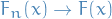 for all continuity points
  of
of  .
. means almost surely convergence for random elements
Theorems
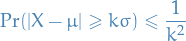
Chebyshev Inequality
Let (integrable) be a random variable with finite expected value  and finite non-zero variance
  .
.
Then for any real number  ,
,
Let  be a measure space, and let
  be an extended real-valued measureable-function defined on .
Then for any real number  and
and 
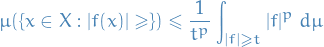
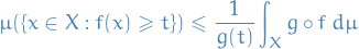
Or more generally, if  is an extended real-valued measurable function, nonnegative and nondecreasing on the range of , then
Hmm, not quite sure how to relate the probabilistic and measure-theoretic definition..
Markov Inequality
If is a nonnegative random variable and  , then
![\begin{equation*}
P \big( X \ge a \big) \le \frac{\mathbb{E}[X]}{a}
\end{equation*}](../../assets/latex/probability_and_statistics_019a98278452845f8b8bb6b44608297d85c8e1a4.png)
First note that
![\begin{equation*}
\mathbb{E}[X] = \int_{0}^{\infty} \mathbb{P}(X \ge t) \dd{t}
\end{equation*}](../../assets/latex/probability_and_statistics_8c1c901415a27fd332fa45ee2e8acb4dbb3c486c.png)
and
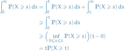
Hence,
![\begin{equation*}
\mathbb{P}(X \ge t) \le \frac{\mathbb{E}[X]}{t}
\end{equation*}](../../assets/latex/probability_and_statistics_fe338901aa40dfd0b5f0c6f1454f4a90f05dc8b9.png)
Law of large numbers
There are mainly two laws of large numbers:

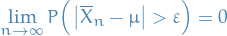
Often the assumption of finite variance is made, but this is in fact not necessary (but makes the proof easier). Large or infinite variance will make the convergence slower, but the Law of Large Numbers holds anyway.
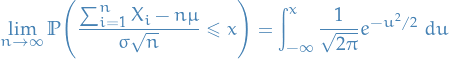
Central Limit Theorem
Suppose  is a sequence of i.i.d. random variables with
 ![$\mathbb{E}[X_i] = \mu$](../../assets/latex/probability_and_statistics_49407bea91d8d9a9fb1131a9ad1c70aa646f9c12.png) and
and  . Then,
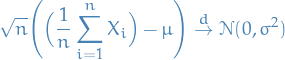
where  means convergence in distribution, i.e. that the cumulative distribution functions of
  converge pointwise to the cdf of the
  distribution: for any real number
  ,
,
![\begin{equation*}
\underset{n \to \infty}{\lim} \Pr [ \sqrt{n} (S_n - \mu) \le z ] = \Phi \Big( \frac{z}{\sigma} \Big)
\end{equation*}](../../assets/latex/probability_and_statistics_93e25db4d6b2ee1fdff8306810f893dd273d7c21.png)
Jensen's Inequality
If
- is a convex function.
- is a rv.
Then ![$f(E[X]) \leq E[f(x)]$](../../assets/latex/probability_and_statistics_5a704c191584b112ce2eae76d3f11effcc23f4d9.png) .
.
Further, if  ( is strictly convex), then
![$E[(f(X)] = f(E[X]) \iff X = E[X]$](../../assets/latex/probability_and_statistics_1a19363be0c70d388d505c858c79d669d8e4944c.png) "with probability 1".
"with probability 1".
If we instead have:
- is a concave function
Then ![$f(E[X]) \geq E[f(X)]$](../../assets/latex/probability_and_statistics_e3025aae464d32e3c1aa1104a8897f1d7c98b121.png) . This is the one we need for the derivation of EM-algorithm.
. This is the one we need for the derivation of EM-algorithm.
To get a visual intuition, here is a image from Wikipedia:

Continuous Mapping Theorem
Let  , be random elements defined on a metric space
  .
.
Suppose a function  (where
  is another metric space) has the set of discountinuity points
  such that
  .
.
Then,


We start with convergence in distribution, for which we will need a particular statement from the
Slutsky's Lemma
Let ,  be sequences of scalarvectormatrix random elements.
If  and
and  , where
  is a constant, then
This follows from the fact that if:
then the joint vector  converges in distribution to
  , i.e.
Next we simply apply the Continuous Mapping Theorem, recognizing the functions
as continuous (for the last mapping to be continuous,  has to invertible).
Definitions
Probability space
A probability space is a measure space  such that the measure of the whole space is equal to one, i.e.
 is the sample space (some arbitrary non-empty set)
 is the σ-algebra over , which is the set of possible events
![$P: \mathcal{A} \to [0, 1]$](../../assets/latex/probability_and_statistics_f7513392d4fb753f764bd899e9b66b18ef63e836.png) which is the probability measure such that
which is the probability measure such that

Random measure
Let  be a separable metric space (e.g.
  ) and let
  be its Borel σ-algebra.
 is a transition kernel from a probability space
  to
to  if
if
For any fixed
 , the mapping

is a measurable function from
 to
to 
For every fixed
 , the mapping
is a (often, probability) measure on
We say a transition kernel is locally finite, if
satisfy  for all bounded measurable sets
  and for all except for some zero-measure set (under
  ).
).
Let be a separable metric space (e.g. ) and let be its Borel σ-algebra.
A random measure is a (a.s.) /locally finite transition kernel from a (abstract) probability space to .
Let be a random measure on the measurable space  and denote the expected value of a random element
  with
with ![$\mathbb{E}[Y]$](../../assets/latex/probability_and_statistics_9e0e384984976b658d0d13ce54607cbf71b8971c.png) .
.
The intensity measure is defined
![\begin{equation*}
\begin{split}
\mathbb{E}\zeta: \quad & \mathcal{A} \to [0, \infty] \\
& A \mapsto \mathbb{E}\zeta(A) := \mathbb{E} \big[ \zeta(A) \big], \quad \forall A \in \mathcal{A}
\end{split}
\end{equation*}](../../assets/latex/probability_and_statistics_5e3283180c137582df4df73bf4f0e9d976dd4389.png)
So it's a non-random measure which sends an element  of the sigma-algebra
  to the expected value of the
  , since is a measurable function, i.e. a random variable.
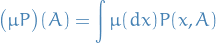
Poisson process
A Poisson process is a generalized notion of a Poisson random variable.
A point process  is a (general) Poisson process with intensity
  if it has the two following properties:
- Number of points in a bounded Borel set
 is a Poisson random variable with mean
  .
.
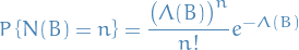
In other words, denote the total number of points located in
by  , then the probability of random variable being equal to
  is given by
- Number of points in disjoint Borel sets form independent random variables.
The Radon measure maintains its previous interpretation of being the expected number of points located in the bounded region , namely
![\begin{equation*}
\Lambda(B) = \mathbb{E} \big[ N(B) \big]
\end{equation*}](../../assets/latex/probability_and_statistics_bf9b7cb287260c314f383ac0bf30d6631f3b9b4b.png)
Cox process
Let be a random measure.
A random measure  is called a Cox process directed by , if
  is a Poisson process with intensity measure .
Here is the conditional distribution of , given  .
.
Degeneracy of probability distributions
A degenerate probability distribution is a probability distribution with support only on a lower-dimensional space.
E.g. if the degenerate distribution is univariate (invoving a single random variable), then it's a deterministic distribution, only taking on a single value.
Characteristic function
Let be a random variable with density  and cumulative distribution function
  .
.
Then the characteristic equation is defined as the Fourier transform of :
![\begin{equation*}
\begin{split}
\varphi_X(t) &= \mathbb{E} \big[ e^{i t X} \big] \\
&= \int_{\mathbb{R}}^{} e^{i t x} \dd{F_X(x)} \\
&= \int_{\mathbb{R}}^{} e^{i t x} f(x) \ \dd{x} \\
&= \mathcal{F} \left\{ f(x) \right\}
\end{split}
\end{equation*}](../../assets/latex/probability_and_statistics_0ae57b2266ee55fcc78f2b1e6a84e6daaceda032.png)
Examples
10 dice: you want at least one 4, one 3, one 2, one 1
Consider the number of misses before a first "hit". When we say "hit", we refer to throwing something in the set  .
.
Then we can do as follows:
 is the # of misses before our first "hit"
 is the # of misses between our first "hit" and second "hit"
- …
We then observe the following:
 since if we have more than
  misses before our first hit, we'll never be able to get all the events in our target set
We also observe that there are  ,
,  ,
,  and
and  ways of missing for each of the respective target events.
from sympy import *

r_1, r_2, r_3, r_4 = symbols("r_1 r_2 r_3 r_4", nonnegative=True, integers=True)

s = Sum(
    Sum(
        Sum(
            Sum(
                (2**(r_1 - 1) * 3**(r_2 - 1) * 4**(r_3 - 1) * 5**(r_4 - 1)) \
                / 6**(r_1 + r_2 + r_3 + r_4),
                (r_4, 1, 10 - r_1 - r_2 - r_3)
            ), (r_3, 1, 9 - r_1 - r_2)
        ), (r_2, 1, 8 - r_1)
    ), (r_1, 1, 7)
)

res = factorial(4) * s.doit()
print(res.evalf())
Probability "metrics" / divergences
Notation
Overview of the "metrics" / divergences
These definitions are taken from arjovsky17_wasser_gan
The Total Variation (TV) distance
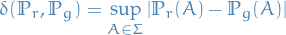
Or, using slightly different notation, the total variation between two probability measures and  is given by
These two notions are completely equivalent. One can see this by observing that any discrepancy between and is "accounted for twice", since  , which is why we get the factor of
  in front. We can then gather all
  where
where  into a subset
  , making sure to choose or it's complement
  such that the difference is positive when in the first term. Then we end up with the
  seen above.
The Jensen-Shannon (JS) divergence

where  is the mixture
  .
.
This divergence is symmetrical and always defiend because we can choose  .
.
The Earth-Mover (EM) distance or Wasserstein-1
![\begin{equation*}
W(\mathbb{P}_r, \mathbb{P}_g) = \inf_{\gamma \in \Pi(\mathbb{P}_r, \mathbb{P}_g)} \mathbb{E}_{(x, y) \sim \gamma} \big[ \norm{x - y} \big]
\end{equation*}](../../assets/latex/probability_and_statistics_4dc254a423d055e723e06f3b67d8f610b955f76c.png)
where  denotes the set of all joint distributions
  whose marginals are respectively
  and
and  .
.
Intuitively, indicates how much "mass" must be transported from to in order to transform the distributions into the distribution . The EM distance then is the "cost" of the optimal transport plan.
Kullback-Leibler divergence
Definition
The Kullback-Leibler (KL) divergence
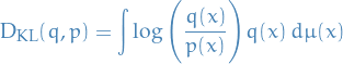
where both  and
and  are assumed to be absolutely continuous, and therefore admit densities, wrt. to the same measure defined on
  .
.
The KL divergence is famously asymmetric and possibly infinite / undefined when there are points s.t.  and
and  .
.
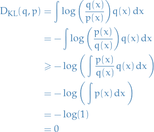
where in the inequality we have use Jensen's inequality together with the fact that  is a convex function.
Why?
Kullback-Leibner divergence from some probability-distributions  and , denoted
  ,
is a measure of the information gained when one revises one's beliefs from the prior distribution
to the posterior distribution . In other words, amount of information lost when
is used to approximate .
,
is a measure of the information gained when one revises one's beliefs from the prior distribution
to the posterior distribution . In other words, amount of information lost when
is used to approximate .
Most importantly, the KL-divergence can be written
![\begin{equation*}
D_{\rm{KL}}(p \ || \ q) = \mathbb{E}_p\Bigg[\log \frac{p(x \mid \theta^*)}{q(x \mid \theta)} \Bigg] = \mathbb{E}_p \big[ \log p(x \mid \theta^*) \big] - \mathbb{E}_p \big[ \log q(x \mid \theta) \big]
\end{equation*}](../../assets/latex/probability_and_statistics_bf4cacc304ab57b5792eb66e803c948e203e94f0.png)
where  is the optimal parameter and
  is the one we vary to approximate
  . The second term in the equation above is the only one which depend on the "unknown" parameter ( is fixed, since this is the parameter we assume
  to take on). Now, suppose we have samples
  from , then observe that the negative log-likelihood for some parametrizable distribution
  is given by
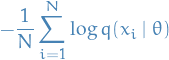
By the Law of Large numbers, we have
![\begin{equation*}
\lim_{N \to \infty} - \frac{1}{N} \sum_{i=1}^{N} \log q(x_i \mid \theta) = - \mathbb{E}_p[\log q(x \mid \theta)]
\end{equation*}](../../assets/latex/probability_and_statistics_96e04ce0e8b58d7c798481548bd91823470368e0.png)
where  denotes the expectation over the probability density . But this is exactly the second term in the KL-divergence! Hence, minimizing the KL-divergence between
  and
and  is equivalent of minimizing the negative log-likeliood, or equivalently, maximizing the likelihood!
Wasserstein metric
Let  be a metric space for which every probability measure on
  is a Radon measure.
For  , let
, let  denote the collection of all probability measures on with finite p-th moment (expectation of rv. to the p-th power) for some
  ,
,
Then the p-th Wasserstein distance between two probability measures and in is defined as
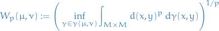
where  denotes the collection of all measures on
  with marginals and on the first and second factors respectively (i.e. all possible "joint distributions").
Or equivalently,
![\begin{equation*}
W_p(\mu, \nu)^p = \inf \mathbb{E} \big[ d(X, Y)^p \big]
\end{equation*}](../../assets/latex/probability_and_statistics_eff0640986bca7f4d56bdce5777eadd3e5f24976.png)
Intuitively, if each distribution is viewed as a unit amount of "dirt" piled on the metric space , the metric minimum "cost" of turning one pile into the other, which is assumed to eb the amount dirt that needs to moved times the distance it has to be moved.
Because of this analogy, the metric is sometimes known as the "earth mover's distance".
Using the dual representation of  , when and have bounded support:

where  denotes the minimal Lipschitz constant for .
Compare this with the definition of the Radon metric (metric induced by distance between two measures):
![\begin{equation*}
\rho(\mu, \nu) := \sup \Bigg\{ \int_M f(x) \dd(\mu - \nu)(x) \mid \text{continuous } f: M \to [-1, 1] \Bigg\}
\end{equation*}](../../assets/latex/probability_and_statistics_4496867e36c7eb7a37a1a4f07a2561baefb11961.png)
If the metric  is bounded by some constant
  , then
and so convergence in the Radon metric implies convergence in the Wasserstein metric, but not vice versa.
Observe that we can write the duality as
![\begin{equation*}
\begin{split}
W_1(\mu, \nu) &= \sup_{\norm{f}_L \le 1} \int_M f(x) \dd (\mu - \nu)(x) \\
&= \sup_{\norm{f}_L \le 1} \int_M f(x) \dd \mu - \int_M f(x) \dd \nu \\
&= \sup_{\norm{f}_L \le 1} \Big( \mathbb{E}_{x \sim \mu(x)} \big[ f(x) \big] - \mathbb{E}_{x \sim \nu(x)} \big[ f(x) \big] \Big)
\end{split}
\end{equation*}](../../assets/latex/probability_and_statistics_15553e9aefcfe1dedcc8397433ee45e41b303211.png)
where we let  denotes that we're finding the supremum over all functions which are 1-Lipschitz, i.e. Lipschitz continuous with Lipschitz constant 1.
Integral Probability Metric
Let and be a probablity distributions, and  be some space of real-valued functions. Further, let
![\begin{equation*}
d_{\mathcal{H}}(q, p) = \sup_{h \in \mathcal{H}} \Big[ \mathbb{E}_q [h(X)] - \mathbb{E}_p[h(Z)] \Big]
\end{equation*}](../../assets/latex/probability_and_statistics_0c6c78693beb9e0630c1502d0c10caca561a8c31.png)
When is sufficently "large", then

We then say that together with  defines an integral probabilty metric (IPM).
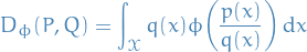
ϕ-divergences
Stein's method
Absolutely fantastic description of it: https://statweb.stanford.edu/~souravc/beam-icm-trans.pdf
Notation
 any random variable
 std. Gaussian random variable
Overview
- Technique for proving generalized central limit theorems
Ordinary central limit theorem: if
are i.i.d. rvs. then
where
 and
and 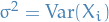
- Usual method of proof:
- LHS is computed using Fourier Transform
- Independence implies that FT decomposes as a product
- Analysis
- Stein's motivation: what if
 are not exactly independent?!
Method
Suppose we want to show that is "approximately Gaussian", i.e.

or,
![\begin{equation*}
\mathbb{E}[h(W)] \approx \mathbb{E}[h(Z)]
\end{equation*}](../../assets/latex/probability_and_statistics_06ba62cf66ccd8f2d07b4e7af4c372d3006f9c65.png)
for any well-behaved 
It's a generalization because if
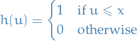
then
![\begin{equation*}
\mathbb{P}(W \le x) = \mathbb{E}[h(W)]
\end{equation*}](../../assets/latex/probability_and_statistics_4b3f596ed4f34ba8748fa9f9529443e4336722a6.png)
Suppose
and we want to show that the rv. is approximately std. Gaussian, i.e. ![$\mathbb{E}[h(W)] \approx \mathbb{E}[h(Z)$](../../assets/latex/probability_and_statistics_519176343a58bbe82f34d8418f7478264192526c.png) for all well-behaved .
for all well-behaved .
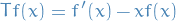
Given
, obtain a function by solving the differential equation
![\begin{equation*}
f'(x) - x f(x) = h(x) - \mathbb{E}[h(z)]
\end{equation*}](../../assets/latex/probability_and_statistics_08424e2fe22e1ee741c245c231dd7f9855374942.png)
2.Show that
![\begin{equation*}
\mathbb{E} \big( f'(W) - W f(W) \big) = \mathbb{E}[h(W)] - \mathbb{E}[h(Z)]
\end{equation*}](../../assets/latex/probability_and_statistics_ed612add542dfee721c1920259327eff80b35f05.png)
using the properties of
Since
![\begin{equation*}
\mathbb{E} \big( f'(W) - W f(W) \big) = \mathbb{E}[h(W)] - \mathbb{E}[h(Z)
\end{equation*}](../../assets/latex/probability_and_statistics_352fb025d181c9a4a0af1ba900d2354c4280269b.png)
conclude that
![$\mathbb{E}[h(W)] \approx \mathbb{E}[h(Z)]$](../../assets/latex/probability_and_statistics_d41733f6a99a480b597c447684432a841ad974c5.png) .
.
More generally, two smooth densities and supported on  are indentical if and only if
![\begin{equation*}
\mathbb{E}_p [\mathbf{s}_p(x) f(x) + \nabla_x f(x) ] = 0
\end{equation*}](../../assets/latex/probability_and_statistics_21eabfd0a3a9afee8f36fed3fff6a71b11356427.png)
for smooth functions  with proper zero-boundary conditions, where
is called the Stein score function of .
Stein discrepancy measure between two continuous densities and is defined
![\begin{equation*}
\mathbb{S}(p, q) = \max_{f \in \mathcal{F}} \big( \mathbb{E}_p [ \mathbf{s}_q(x) f(x) + \nabla_x f(x)] \big)^2
\end{equation*}](../../assets/latex/probability_and_statistics_f88b77c8cb9a1b198313c15cbf27b3e14a1ef50c.png)
where  is the set of functions which satisfies
Two smooth densities and supported on are indentical if and only if
![\begin{equation*}
\mathbb{E}_p [\mathbf{s}_q(x) f(x) + \nabla_x f(x) ] = 0
\end{equation*}](../../assets/latex/probability_and_statistics_bc24722f15cc69291023190e774861f5f083e897.png)
for smooth functions with proper zero-boundary conditions, where
is called the Stein score function of .
Stein discrepancy measure between two continuous densities and is defined
where is the set of functions which previous expectation and is also "rich" enough to ensure that  whenever
  .
.
Why does it work?
- Turns out that if we replace the
![$\mathbb{E}[h(Z)]$](../../assets/latex/probability_and_statistics_94d7d167dd4ca6ec844eb249c4e3e3b5f0be774c.png) in Stein's method, then is not well-behaved; it blows up at infinity.
in Stein's method, then is not well-behaved; it blows up at infinity. - A random variable has the standard Gaussian distribution if and only if
 for all !
(you can easilty check this by observing that the solution to this is
for all !
(you can easilty check this by observing that the solution to this is  ).
). Differential operator
 , defined as
is called a characterizing operator for the standard Gaussian distribution.
Stochastic processes
Discrete
- Markov chains is an example of a discrete stochastic process
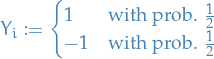
Simple random walk
Let  be a set of i.i.d. random variables such that
Then, let
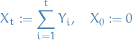
We then call the sequence  a simple random walk.
For large  , due to CLT we have
i.e.  follows a normal distribution with
 ![$\mathbb{E}[X_t] = 0$](../../assets/latex/probability_and_statistics_d3e8c75430646506718908bbc841c0b1bb0b8eef.png) and
and  .
.
We then have the following properties:
![$\mathbb{E}[X] = 0$](../../assets/latex/probability_and_statistics_56be98dff9b0eedfc7b4bba0860fc3638ddd82e1.png)
Independent measurements : if

then
 are mutually independent, with
  .
.
- Stationary : for all
 and
and  , the distribution of
  is the same as the distribution of
  .
.
Martingale
A martingale is a stochastic process which is fair game.
We say a stochastic process  is a martingale if
![\begin{equation*}
X_t = \mathbb{E}[X_{t + i} \mid \mathcal{F}_t], \quad i \ge 0
\end{equation*}](../../assets/latex/probability_and_statistics_270a8ecf4eafe631538496cac4746d3846577297.png)
where
Examples
- Simple random walk is a martingale
- Balance of a Roulette player is NOT martingale
Optional stopping theorem
A given stochastic process  , a non-negative integer r.v.
  is called a stopping time if

depends only on  (i.e. stopping at some time only depends on the first
  r.v.s).
 is
is  , and
, and
![\begin{equation*}
\mathbb{E}[X_{\tau}] = X_0
\end{equation*}](../../assets/latex/probability_and_statistics_cc5d570588453c1c6a2ae039f13292fbb9eaf912.png)
This implies that if we a process can be described as a martingale, then it's a "zero-sum".
Continuous
Lévy process
A stochastic process  is said to be a Lévy process if it satisfies the following properties:
 almost surely.
- Independence of increments: for any $0 ≤ t1 ≤ t2 ≤ … ≤ tn < ∞, the increments
 are independent.
 - Stationary increments: For any
 , the rvs.
  is equal in distribution to
  .
. Continuity in probability: For any
 and it holds that
If is a Lévy process then one may construct a version of such that  is almost surely right-continuous with left limits.
Wiener process
The Wiener process (or Brownian motion) is a continuous-time stochastic process  characterized by the following properties:
 (almost surely)
- has independent increments: for , future increments
 with
with  , are independent of the past values
  ,
, 
- has Gaussian increments:
- has continuous paths: with probability
 , is continuous in
Further, let  be i.i.d. rv. with mean 0 and variance 1. For each , define the continuous-time stochastic process
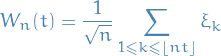
Then

i.e. a random walk approaches a Wiener process.
Properties
 .
.
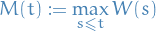
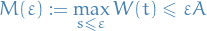
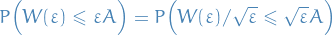
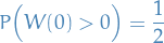
Let  be the first time such that

Then
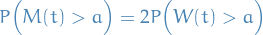
Observe that

which is saying that at the point we have  , and therefore for all time which follows we're equally likely to be above or below
  .
.
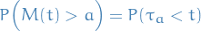
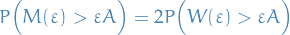
Therefore
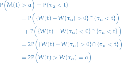
where in the last inequality we used the fact that the set of events  .
.
This theorem helps us solve the gambler's ruin problem!
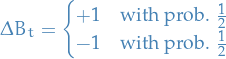
Let  denote your bankroll at time , and at each it changes by
The continuous approximation of this process is given by a Brownian motion, hence we can write the bankroll as
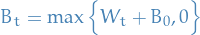
where denotes a Brownian motion (with ![$\mathbb{E}[W_t] = 0$](../../assets/latex/probability_and_statistics_7a7e0761a608ecf7946800a88f5b331d904e6ff3.png) ).
).
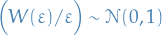
We're interested in how probable it is for us to be ruined before some time . Letting be the time were we go bankrupt, we have
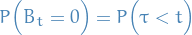
i.e. that we hit the time were we go bankrupt before time .
Bankrupt corresponds to

where denotes a Wiener process (hence centered at 0).
Then we can write

where the last equality is due to the symmetry of a Normal distribution and thus a Brownian motion.
Hence

where  denotes a standard normal distribution.
![\begin{equation*}
\lim_{n \to \infty} \Big[ B \Big(T (t / n) \Big) - B\Big(T (t - 1) / n \Big) \Big]^2 = T
\end{equation*}](../../assets/latex/probability_and_statistics_d2676857ceb9dd02ba9d8dd6aa20b7abc46bcd3c.png)
This is farily straightforward to prove, just recall the Law of Large numbers and you should be good.
Non-differentiability
 is non-differentiable with probability 1.
Suppose, for the sake of contradiction, that is differentiable with probability 1.
Then, by MVP we have

for some and all . This implies that
since  .
.
Hence
As  , since
  , then
where
Thus, when , we have
since 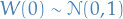 Hence,
contracting our initial statement.
Geometric Brownian motion
A stochast process  is said to follow a Geometric Brownian Motion if it satisfies the following stochastic differential equation (SDE):

where is the Brownian motion, and (percentage drift) and  (percentage volatility) are constants.
Brownian bridge
A Brownian bridge is a continuous-time stochastic process  whose probability distribution is the conditional probability distribution of a Brownian motion subject to the condition that

so that the process is pinned at the origin at both  and
and  . More precisely,
![\begin{equation*}
B_t := \big( W_t \mid W_T = 0 \big), \quad t \in [0, T]
\end{equation*}](../../assets/latex/probability_and_statistics_8238711534767675a010b92c07f261a709260728.png)
Then
![\begin{equation*}
\mathbb{E}[B_t] = 0, \quad \text{Var}(B_t) = \frac{t (T - t)}{T}
\end{equation*}](../../assets/latex/probability_and_statistics_400aba49f998227142fefa7ee51e38a6da33a6af.png)
implying that the most uncertainty is in the middle of the bridge, with zero uncertainty at the nodes.
Sometimes the notation is used for a Wiener process / Brownian motion rather than for a Brownian bridge.
Markov Chains
Notation
- denotes the transition matrix (assumed to be ergodic, unless stated otherwise)
 is the stationary distribution
 denotes the initial state
- is the state space
- denotes an uncountable state space
 denotes
  which means all points except those with zero-measure, i.e.
  such that
Definitions
A Markov chain is said to be irreducible if it's possible to reach any state from any state.
A state  has a period if any return to state must occur in multiples of time steps.
Formally, the period of a state is defined as

provided that the set is non-empty.
A state is said to be transient if, given that we start in state ,t there is a non-zero probability that we will never return to .
A state is said to be recurrent (or persistent) if it is not transient, i.e. gauranteed (with prob. 1) to have a finite hitting time.
A state is said to be ergodic if it is aperiodic and positive recurrent, i.e.
- aperiodic: period of 1, i.e. can return to current state in a single step
- positive recurrent: has a finite mean recurrence time
If all states in an irreducible Markov chain are ergodic , then the chain is said to be ergodic.
The above definitions can be generalized to continuous state-spaces by considering measurable sets  rather than states . E.g. recurrence now means that for any measurable set , we have
where  denotes the number of steps we need to take until we "hit" , i.e. the hitting time.
[This is a personal thought though, so not 100% guaranteed to be correct.]
Coupling
- Useful for bouding the mixing rate of Markov chains, i.e. the number of steps it takes for the Markov chain to converge to the stationary distribution
Distance to Stationary Distribution
Use Total Variance as a distance measure, therefore convergence is defined through
 denotes the variation distance between two Markov chain random variables
  and
and  , i.e.
One can prove that
which allows us to bound the distance between a chain and the stationary distribution, by considering the difference between two chains, without knowing the stationary distribution!
Coupling
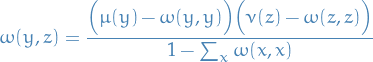
Let and be random variables with probability distributions and on , respectively.
A distribution  on
on  is a coupling if
Consider a pair of distributions and on .
For any coupling
of and , with 

There always exists a coupling
s.t.
Observe that

Therefore,
Concluding the proof.
"Inspired" by our proof in 1., we fix diagonal entries:

to make one of the inequalities an equality. Now we simply need to construct
such that the above is satisfied, and it's a coupling. One can check that
does indeed to the job.
Ergodicity Theorem
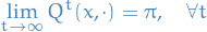
If is irreducible and aperiodic, then there is a unique stationary distribution such that
Consider two copies of the Markov chain and  , both following . We create the coupling distribution as follows:
- If
 , then choose
  and
and  independently according to
 - If
 , choose
  and set
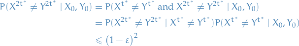
From the couppling lemma, we know that

Due to ergodicity, there exists  such that
  . Therefore, there is some such that for all initial states
  and
and  ,
,

Similarily, due to the Markovian property, we know

Since

we have
Hence, for any positive integer :

Hence,

Coupling lemma then gives
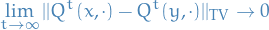
Finally, we observe that, letting 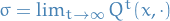 ,
,
which shows that  , i.e. converges to the stationary distribution.
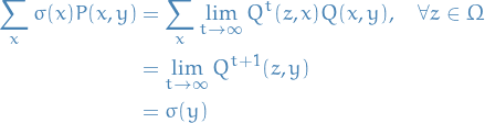
Finally, observe that is unique, since

Mixing time
Let be some  and let have the stationary distribution. Fix .
By the coupling lemma, there is a coupling and random variables
and let have the stationary distribution. Fix .
By the coupling lemma, there is a coupling and random variables  and
and  such that

Using this coupling, we define a coupling of the distributions of  as follows:
- If
 , set
, set 
- Else, let
 and
and  independently
Then we have,

The first inequality holds due to the coupling lemma, and the second inequality holds by construction of the coupling.
Since  never decreases, we can define the mixing time
  of a Markov chain as
for some chosen .
General (uncountable) state space
Now suppose we have some uncountable state-space . Here we have to be a bit more careful when going about constructing Markov chains.
- Instead of considering transitions
 for some
  , we have to consider transitions
  for and
  .
.
- Transition probability is therefore denote

- Transition probability is therefore denote
- This is due to the fact that typically, the measure of a singleton set
 is zero, i.e.
  , when we have an uncountable number possible inputs.
 - That is; we have to consider transitions to subsets of the state-space, rather than singletons
- This requires a new definition of irreducibility of a Markov chain
A chain is  if there exists a non-zero sigma-finite measure
  on such that for all
  with
with  (i.e. all non-zero measurable subsets), and for all , there exists a positive integer
  such that
We also need a slightly altered definition of periodicity of a Markov chain:
A Markov chain with stationary distribution is periodic if there exist  and disjoint subsets
  with
with

and
such that  , and hence
  for all . That is, we always transition between subsets, and never within these disjoint subsets.
If such does not exist, i.e. the chain is not periodic, then we say the chain is aperiodic.
Results such as the coupling lemma also hold for the case of uncountable state-space, simply by replacing the summation with the corresponding integrand over the . From roberts04_gener_state_space_markov_chain_mcmc_algor, similarily to the countable case, we have the following properties:
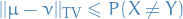
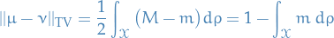
Let and be probability measures on the space . Then
![$||\mu - \nu||_{\rm{TV}} = \sup_{f : \mathcal{X} \to [0, 1]} \left| \int f d \mu - \int f d \nu \right|$](../../assets/latex/probability_and_statistics_381334c21ab2d08946d2920a57405b378136dc70.png)
More generally,
![\begin{equation*}
||\mu - \nu||_{\rm{TV}} = \frac{1}{b - a} \sup_{f: \mathcal{X} \to [a, b]} \left| \int f \ d \mu - \int f \ d \nu \right|
\end{equation*}](../../assets/latex/probability_and_statistics_7f1df4fa4639c3eac471ad5d77867381654a9621.png)
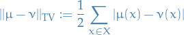
In particular,
![\begin{equation*}
||\mu - \nu||_{\rm{TV}} = \frac{1}{2} \sup_{f: \mathcal{X} \to [-1, 1]} \left| \int f \ d \mu - \int f \ d \nu \right|
\end{equation*}](../../assets/latex/probability_and_statistics_5fc1b80015a31e2ab01be527365a3eb8647b7be4.png)
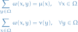
If
is a stationary distribution for a Markov chain with kernel , then  is non-increasing in , i.e.

for
 .
.
More generally, letting
we always have

If
and have densities and , respectively, wrt. to some sigma-finite measure  , then
with

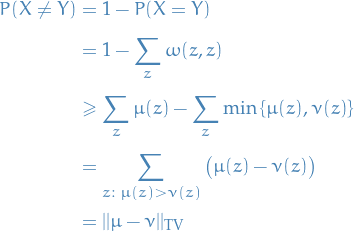
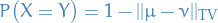
Given probability measures
and , there are jointly defined random variables and such that
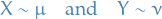
and
From roberts04_gener_state_space_markov_chain_mcmc_algor we also have the following, important theorem:
If a Markov chain on a state space with countable generated sigma-algebra is irreducible and aperiodic, and has a stationary distribution , then for almost-every ,
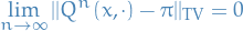
In particular,

We also introduce the notion of Harris recurrent:
We say a Markov chain is Harris recurrent if for all  with
with  (i.e. all non-zero-measurable subsets), and all , the chain will eventually reach from with probability 1, i.e.

This notion is stronger than the notion of irreducibility introduced earlier.
Convergence rates
Uniform Ergodicity
From this theorem, we have implied asymptotic convergence to stationarity, but it does not provide us with any information about the rate of convergence. One "qualitative" convergence rate property is
A Markov chain having stationary distribution is uniformly ergodic if

for some  and
and  .
.
For further developments of ensuring uniform ergodicity, we need to define
A subset  is small or
  if there exists a positive integer
  , , and a probability measure on s.t. the following minorisation condition holds:

i.e. 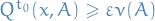 for all
  and all measurable .
Geometric ergodicity
A Markov chain with stationary distribution is geometrically ergodic if

for some where  for
for  .
.
Difference between uniform ergodicity and geometric ergodicity is the fact that in geometric ergodicity the can also depend on the initial state .
In practice
Diagnostics
Effective sample size (ESS)
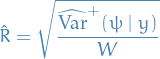
(split)  statistic
- Consider running
 chains, each for
  steps, from different initializations , where
  is even
 - Then consider splitting each chain in half, resulting in two half-chains for each chain, leaving us with a total of
 chains
- Reason: If a chain indeed represents independent samples from the stationary distribution, then at the very least the first half and second half of the chain should indeed have the display similar behavior (for sufficiently large )
- Reason: If a chain indeed represents independent samples from the stationary distribution, then at the very least the first half and second half of the chain should indeed have the display similar behavior (for sufficiently large
You might wonder, why not split in 3? Or 4? or, heck,  ?!
?!
Likely answer: "You could, but be sensible!" Very unsatisfying…
Let  be the scalar estimand, i.e. the variable we're trying to estimate. Let
  be the "for
  and
and  denote the different samples for the variable of interest obtained by MCMC chains, each with samples each, with different initializations.
We denote the (B)etween- and (W)ithin-sequence variances
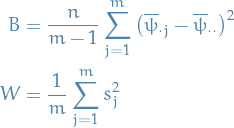
where
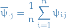
empirical mean within a chain
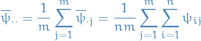
empirical mean across all chains
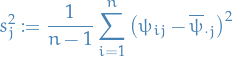
empirical variance within each chain
Notice that contains a factor of because it is based on the variance of the within-sequence means  , each of which is an averaeg of values .
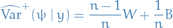
We can then estimate  , the marginal posterior variance of the estimand, by a weighted average of and , namely
Finally, we can then monitor convergence of the iterative simulation by estimating the factor by which the scale of the current distribution for might be reduced if the simulations were continued in the limit  . This potential scale reduction is estimated by
which has the property that

(remember that  depend on ).
If
- is large → reason to believe that further simulations may improve our inference about the target distribution of the associated scalar estimand
- is small → ???
Specific distributions & processes
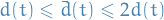
Hazard function
The hazard function / failure rate  is defined
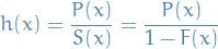
where denotes the PDF and denotes the CDF.
TODO Renewal processes
- Let
 with
with  be a sequence of waiting times between
  and the
  event.
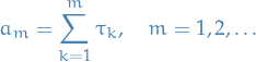
 Arrival time of the
 event is
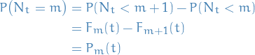
- Denote by the total number of events in

- If is fixed, then
 is the count variable we wish to model
It follows that

i.e. total number of events is less than
if and only if the arrival time of the  event is greater than , which makes sense
If
 is the distribution function of
  , we have

Furthermore
- This is the fundamental relationship between the count variable and the timing process
- This is the fundamental relationship between the count variable
- If
 , the process is called a renewal process
 In this case, we can extend the above equation to the following recursive relationship:
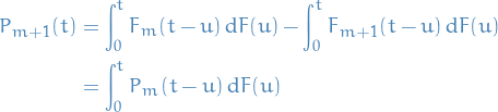
where we have

- Intuitively: probability of exactly
 events occuring by time is the probability that the first event occurs at time
  , and that exactly events occur in the remaining time interval, integrated over all times
  .
. - Evaluting this integral, we can obtain
 from the above recursive relationship.
- Intuitively: probability of exactly
Weibull renewal process
Statistics
Notation
 denotes converges in probability to
  denotes convergence in law to
Definitions
Efficency
The efficency of an unbiased estimator  is the ratio of the minimum possible variance to
  .
.
An unbiased estimator with efficiency equal to 1 is called efficient or a minimum variance unbiased estimator (MVUE).
Statistic
Suppose a random vector  has distribution function in a parametric family
  and realized value
  .
.
A statistic is r.v.  which is a function of independent of . Its realized value is
  .
.
A statistic is said to be sufficient for if the distribution of given does not depend on , i.e.
Further, we say is a minimal sufficient statistic if it's the smallest / least complex "proxy" for .
Observe that,
- if is sufficient for , so is any one-to-one function of
- is trivially sufficient
We say a statistic is pivotal if it does not depend on any unknown parameters.
E.g. if we are considering a normal distribution  and is known, then the mean could be a pivotal statistic, since we know all information about the distribution except the statistic itself. But if we didn't know , the mean would not be pivotal.
Let  .
.
Then statistic 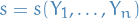 is sufficient for if and only if there exists functions of and of
  such that

where  denotes the likelihood.
U-statistic
Let be independent observations on a distribution .
Consider a "parametric function"  for which there is an unbiased estimator. That is,
  may be represented as
![\begin{equation*}
\theta(F) = \mathbb{E}_F \big[ h(X_1, \dots, X_m) \big] = \int \dots \int h(x_1, \dots, x_m) \dd{F(x_1)} \cdots \dd{F(x_m)}
\end{equation*}](../../assets/latex/probability_and_statistics_d65325ac98ad0431810d295a5d19bfb7fe5b58ee.png)
for some function 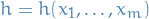 , called a kernel.
Without loss of generality, we may assume is symmetric, otherwise we could simply
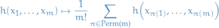
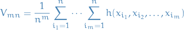
For any kernel , the corresponding U-statistic for estimation of on the basis of a sample  for size
  is obtained by averaging the kernel symmetrically over the observations:
where  denotes the summation over
  combinations of distinct elements
  from
from  .
.
Clearly,  is then an unbiased estimate of .
To conclude, a U-statistic is then a statistic which has the property of being an unbiased estimator for the corresponding , where is such that it can be written stated above.
V-statistic
Statistics that can be represented as functionals  of the empirical distribution function,
  , are called statistical functionals.
A V-statistic is a statistical function (of a sample) defined by a particular statistical functional of a probability distribution.
Suppose  is a sample. In typical applications the statistical function has a representation as the V-statistic
where is a symmetric kernel function.
 is called a V-statistic of degree .
Seems very much like a form of boostrap-estimate, does it not?
Informally, the type of asymptotic distribution of a statistical function depends on the order of "degeneracy," which is determined by which term is the first non-vanishing term in the Taylor expansion of the functional .
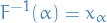
Quantiles
Let be a random variable with cumulative density function (CDF) , i.e.
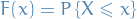
Let  be such that
for some ![$\alpha \in [0, 1]$](../../assets/latex/probability_and_statistics_df706ca088cfab3f5c3067f3ca880bfddf0f6fa5.png) .
.
Then we say that is called the  quantile of , i.e. the value such that

We then say:
 is the median; half probability mass on each side
 is the lower quantile
 is the upper quantile
is strictly monotonically increasing so  exists, hence we can compute the quantiles!
Convergence in law
A sequence of cdfs  is said to converge to
  iff
iff 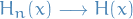 on all continuity points of .
We say that if a random variable  has cdf and the rv has cdf , then converges in law to , and we write

This does not mean that and are arbitrarily close as random variables. Consider the random variables  and
and  .
.
Let and be random variables. Then

where  means converges in probability.
Or, equivalently

This is the notion used by WLLN.
If  where is the limit distribution and
  then
then

Let  be a sequence of random variables, and be a random variable.
Then
This is the notion of convergence used by SLLN.
Kurtosis
The kurtosis of a random variable is the 4th moment, i.e.
![\begin{equation*}
\text{Kurt}[X] = \kappa(X) = \mathbb{E} \Bigg[ \bigg( \frac{X - \mu}{\sigma} \bigg)^4 \Bigg] = \frac{\mu_4}{\sigma^4} = \frac{\mathbb{E}[(X - \mu)^4]}{\big(\mathbb{E}[(X - \mu)^2]\big)^2}
\end{equation*}](../../assets/latex/probability_and_statistics_999127ed41a92556298ca94fe627e7880cb44028.png)
where  denotes the 4th central moment and is the std. dev.
Words
A collection of random variables is homoskedastic if all of these random variables have the same finite variance.
This is also known as homogeneity of variance.
A collection of random variables is heteroskedastic if there are sub-populations that have different variability from others.
Thus heteroskedasticity is the absence of homoskedastic.
Consistency
Loosely speaking, an estimator  of parameter is said to be consistent, if it converges in probability to the true value of the parameter:

Or more rigorously, suppose  is a family of distributions (the parametric model) and
  is an infinite sample from the distribution
  .
.
Let  be a sequence of estimators for some parameter
  . Usually will be based on the first observations of a sample. Then this sequence is said to be (weakly) consistent if
Jeffreys Prior
The Jeffreys prior is a non-informative prior distribution for a parameter space, defiend as:
It has the key feature that it is invariant under reparametrization.
Moment generating function
For r.v. the moment generating function is defined as
![\begin{equation*}
M_x(t) = \mathbb{E} [e^{tX}], \quad t \in \mathbb{R}
\end{equation*}](../../assets/latex/probability_and_statistics_478db7622be48bf5634482c422f45780b09638e0.png)
Taking the derivative wrt. we observe that
![\begin{equation*}
\frac{\partial M_x}{\partial t} = \mathbb{E}[X e^{tX}]
\end{equation*}](../../assets/latex/probability_and_statistics_b737676d842bc4dfef42eab4fb0aaf297a3623ba.png)
Letting  , we get
![\begin{equation*}
\frac{\partial M_x}{\partial t} = \mathbb{E}[X]
\end{equation*}](../../assets/latex/probability_and_statistics_e540fafcfcf7bb424d3e256240d9ee11a3f94635.png)
i.e. the mean. We can take this derivative times to obtain the expectation of  , which is why
  is useful.
Distributions
Binomial

or equivalently,
Negative binomial
A negative binomial random variable represents the number of success before obtaining  failures, where is the probability of a failure for each of these binomial rvs.
Derivation
Let  denote the rv. for # of successes and
  the number of failures.
Suppose we have a run of  successes and
  failure, then

where the failure is of course the last thing that happens before we terminate the run.
Now, suppose that the run above is followed up by  failures, i.e.
  but we have a specific ordering. Then, letting
  denote the result of the i-th Binomial trail,

But for of the failures, we don't actually care when they happen, so we don't want any ordering. That is, we have  sequences of the form described above which are acceptable.
Hence we get the pmf
Gamma distribution
Chi-squared distribution
The chi-squared distribution with degrees of freedom is the distribution of a sum of the squares of independent standard normal random variables.
It's a special case of the gamma distribution.
T-distribution
The T-distribution arises as a result of the Bessel-corrected sample variance.
Why?
Our population-model is as follows:
Let
then let
be the Bessel-corrected variance. Then the random variable
and the random variable

(where has been substituted for ) has a Student's t-distribution with  degrees of freedom.
Note that the numerator and the denominator in the preceding expression are independent random variables, which can be proved by a simple induction.
F-distribution
A random variate of the F-distribution with parameters  and
and  arises as the ratio of the two appropriately scaled chi-quared variates:

where
 and
and  have a chi-squared distribution with and degrees of freedom respectively
- and are independent
Power laws
Notation
 such that we have a power law
  , in such cases we say that the tail of the distribution follows a power law
Definition
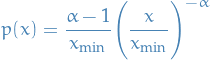
A continuous power-law is one described by probability density such that

where is the observed value and is the normalization constant. Clearly this diverges as  , hence cannot hold for all
  ; must be a lower bound to power-law behavior.
Provided  , we have
A discrete power-law is defined by

Again, diverges at zero, hence must be some lb  on power-law behaviour:
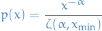
where
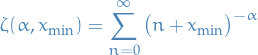
is the generalized or Hurwitz zeta function.
Important
Sources: clauset07_power_law_distr_empir_data and so_you_think_you_have_a_power_law_shalizi
- Log-log plot being roughly linear is necessary but not sufficient
- Errors are hard to estimate because they are not well-defined by the usual regression formulas, which are based on assumptions that do not apply in this case: noise of logarithm is not Gaussian as assumed by linear regression. In continuous case, this can be made worse by choice of binning scheme used to construct histogram, hence we have an additional free parameter.
- A fit to a power-law distribution can account for a large fraction of the variance even when fitted data do not follow a power law, hence high values of
 ("explained variance by regression fit") cannot be taken as evidence in favor of the power-law form.
 - Fits extracted by regression methods usually do not satisfy basic requirements on probability distributions, such as normalization and hence cannot be correct.
- Abusing linear regression. Standard methods, e.g. least-squares fitting are known to produce systematically biased estimates of parameters for power-law distributions and should not be used in most circumstances
- Use MLE to estimate scaling exponent
- Use goodness of fit to estimate scaling regions.
- In some cases there are only parts of the data which actually follows a power law.
- Method based on Kolmogorv-Smirnov goodness-of-fit statistic
- Use goodnes-of-fit test to check goodness of fit
- E.g. Kolmogorov-Smirnov test to check data drawn from estimated power law vs. real data
- Use Vuong's test to check for alternative non-power laws (see likelihood_ratio_test_for_model_selection_and_non_nested_hypothesis_vyong89)
![\begin{equation*}
\hat{\alpha} = 1 + n \Bigg[ \sum_{i=1}^{n} \ln \bigg( \frac{x_i}{x_{\text{min}}} \bigg) \Bigg]
\end{equation*}](../../assets/latex/probability_and_statistics_d8a4d2a65ef8ba890eae5d9d647be1ca78498eb1.png)
Maximum Likelihood Estimation
Notation
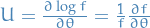
 denotes the log-likelihood , i.e.
 is the Fisher's information (expected information)
 is the observed information , i.e. information without taking the expectation
 is called the score function
 denotes that true (and thus unobserved) parameter
 means the probability density
  evaluated at
Appoximate (asymptotic) variance of MLE
For large samples (and under certain conditions ) the (asymptotic) variance of the MLE is given by
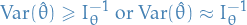
where
![\begin{equation*}
I_\theta = \mathbb{E} \Bigg( \Bigg[ \frac{dl}{d\theta} \Bigg]^2 \Bigg) = - \mathbb{E} \Bigg( \frac{d^2 l}{d\theta^2} \Bigg)
\end{equation*}](../../assets/latex/probability_and_statistics_c6026d15fa470bb7097a7a0dde8138840c1a4282.png)
where is called the Fisher information .
Estimated standard error
The estimated standard error of the MLE of is given by
Regularity conditions
The lower bound of the variance of the MLE is true under the following conditions on the probability density function,  , and the estimator
  :
:
- The Fisher information is always defined; equivalently for all such that
 :
:
exists and is finite.
- The operations of integration wrt. to and differentiation wrt. can be interchanged in the expectation of ; that is,
![\begin{equation*}
\frac{\partial}{\partial \theta} \Bigg[ \int T(x) f(x;\theta) \ dx \Bigg] = \int T(x) \Big[ \frac{\partial}{\partial \theta} f(x; \theta) \Big] \ dx
\end{equation*}](../../assets/latex/probability_and_statistics_6c64d356fe0aa2961efd3466b02125c5a6e1c96a.png)
whenever the RHS is finite. This condition can often be confirmed by using the fact that integration and differentiation can be swapped when either of the following is true:
- The function has bounded support in , and the bounds do not depend on
- The function has infinite support, is continuously differentiable, and the integral converges uniformly for all
Proof (single variable)
"Proof" (alternative, also single variable)
- Notation
 denotes the expectation over the data , assuming the data arises from the model specified by the parameter
  is the same as above, but assuming
 denotes the score, where we've made the dependence on the data explicit by including it as an argument
- Stuff
- Consistency of as an estimator
Suppose the true parameter is
, that is:
Then, for any
 (not necessarily ), the Law of Large Numbersimplies the convergence in probability
![\begin{equation*}
\frac{1}{n} \sum_{i=1}^{n} \log f(X_i \mid \theta) \to \mathbb{E}_{\theta_0}[\log f(X \mid \theta)]
\end{equation*}](../../assets/latex/probability_and_statistics_38a1afa016cb0802911d69d3fb99b6c48d855b5c.png)
Under suitable regularity conditions, this implies that the value of
maximizing the LHS, which is , converges in probability to the value of maximizing RHS, which we claim is .
Indeed, for any
![\begin{equation*}
\mathbb{E}_{\theta_0}[ \log f(X \mid \theta)] - \mathbb{E}_{\theta_0} [ \log f(X \mid \theta_0)] = \mathbb{E}_{\theta_0} \Bigg[ \log \frac{f(X \mid \theta)}{f(X \mid \theta_0} \Bigg]
\end{equation*}](../../assets/latex/probability_and_statistics_8a065868d54f7d3f27f9eaa55dee2843d2a54aa5.png)
Noting that
 is concave, Jensen's Inequality implies
![\begin{equation*}
\mathbb{E}[\log X] \le \log \mathbb{E}[X]
\end{equation*}](../../assets/latex/probability_and_statistics_c3d09c146a6ce43fab76633e4dfca4ca0d6f58cd.png)
for any positive random variable
, so
![\begin{equation*}
\begin{split}
\mathbb{E}_{\theta_0}\Bigg[ \log \frac{f(X \mid \theta)}{f(X \mid \theta_0)} \Bigg] & \le \log \mathbb{E}_{\theta_0} \Bigg[ \frac{f(X \mid \theta)}{f(X \mid \theta_0)} \Bigg] \\
& = \log \int \frac{f(x \mid \theta)}{f(x \mid \theta_0)} f(x \mid \theta_0) \ dx \\
&= \log \int f(x \mid \theta_0) \ dx \\
&= 0
\end{split}
\end{equation*}](../../assets/latex/probability_and_statistics_0ed41b771f87ebc4eb100285a0baf81662be5549.png)
Which establishes "consistency" of
since ![$\theta \mapsto \mathbb{E}_{\theta_0}[\log f(X \mid \theta)]$](../../assets/latex/probability_and_statistics_95959728964caee763d8ae36db8189c9c744e019.png) is maximized at
is maximized at  .
.
- Expectation and variance of score
For
,
![\begin{equation*}
\mathbb{E}_{\theta}[U(X, \theta)] = 0, \qquad \text{Var}_{\theta} \big( U(X, \theta) \big) = - \mathbb{E}[U'(X, \theta)]
\end{equation*}](../../assets/latex/probability_and_statistics_64bc641e48dae229ceb7b967982458f04c4273ae.png)
First, for the expectation we have
![\begin{equation*}
\begin{split}
\mathbb{E}_{\theta}[U] &= \int U(x, \theta) f(x; \theta) \ dx \\
&= \int \Bigg( \frac{\partial \log f(x; \theta)}{\partial \theta} \Bigg) f(x; \theta) \ dx \\
&= \int \Bigg( \frac{1}{f(x; \theta)} \frac{\partial f}{\partial \theta} \Bigg) f(x; \theta) \ dx \\
&= \int \frac{\partial f}{ \partial \theta} \ dx
\end{split}
\end{equation*}](../../assets/latex/probability_and_statistics_2992b8afaa3afeabbdde632f36d8abfb74e8a772.png)
Assuming we can interchange the order of the derivative and the integral (which we can for analytic functions), we have
![\begin{equation*}
\begin{split}
\mathbb{E}_{\theta}[U(X, \theta)] &= \frac{\partial}{\partial \theta} \int f(x; \theta) \ dx \\
&= \frac{\partial}{\partial \theta} \big( 1 \big) \\
&= 0
\end{split}
\end{equation*}](../../assets/latex/probability_and_statistics_e875f5d9ee6249a92e736ef5d54ef78f91fa04d6.png)
For the variance, we can differentiate the above identity:
![\begin{equation*}
\begin{split}
0 &= \frac{\partial}{\partial \theta} \mathbb{E}_{\theta}[U] \\
&= \frac{\partial}{\partial \theta} \int U(x, \theta) f(x \mid \theta) \ dx \\
&= \int U'(x, \theta) f(x \mid \theta) + U(x, \theta) \Big( \frac{\partial}{\partial \theta} f(x \mid \theta) \Big) \ dx \\
&= \int U'(x, \theta) f(x \mid \theta) \ dx + \int U(x, \theta) \Big( U(x, \theta) f(x \mid \theta) \Big) \ dx \\
&= \int U'(x, \theta) f(x \mid \theta) \ dx + \int U^2 f(x \mid \theta) \ dx \\
&= \mathbb{E}_{\theta}[U'] + \mathbb{E}_{\theta}[U^2] \\
&= \mathbb{E}_{\theta}[U'] + \text{Var}_{\theta}(U^2)
\end{split}
\end{equation*}](../../assets/latex/probability_and_statistics_0c91422235ea46c6b9b99425dbd18573eb2ecebd.png)
where we've used the fact that
 and
and ![$\mathbb{E}_{\theta}[U] = 0$](../../assets/latex/probability_and_statistics_01a6c4156e5615ab2aa85e4d2d4df02bc654b0f5.png) , which implies that
, which implies that ![$\text{Var}_{\theta}(U) = \mathbb{E}_{\theta}[U^2]$](../../assets/latex/probability_and_statistics_a5e3956f996d406f4942a9948347f460d0275fcb.png) .
.
This is equivalent to
![\begin{equation*}
\text{Var}_{\theta}(U^2) = - \mathbb{E}_{\theta}[U']
\end{equation*}](../../assets/latex/probability_and_statistics_dfafe59504c65eb46349a7c5653e73f1b550e663.png)
as wanted.
- Asymptotic behavior
Now, since
maximizes  , we must have
  .
.
Consistency of
ensures that is close to (for large n, with high probability). Thus, we an apply first-order Taylor expansion to the equation about the point :

Thus,
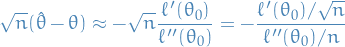
For the denominator, we rewrite as
![\begin{equation*}
\begin{split}
\frac{1}{n} \ell''(\theta_0) &= \frac{1}{n} \sum_{i=1}^{n} \frac{\partial^2}{\partial \theta^2} \Big[ \log f(X_i \mid \theta) \Big]_{\theta = \theta_0} \\
&= \sum_{i=1}^{n} U'(X_i, \theta_0)
\end{split}
\end{equation*}](../../assets/latex/probability_and_statistics_3b26ab2d3e5b7f61665190bffbd702825448448f.png)
and then, by the Law of Large Numbers again, we have
![\begin{equation*}
\sum_{i=1}^{n} U'(X_i, \theta_0) \overset{p}{\to} \mathbb{E}_{\theta_0}[U(X, \theta_0)] = - I(\theta_0)
\end{equation*}](../../assets/latex/probability_and_statistics_4efb018bcb2e4d08fdd85c272f40a87792a9d62c.png)
in probability.
For the numerator, due to what we showed earlier, we know that
![\begin{equation*}
X \sim f(x \mid \theta_0) \quad \implies \quad \mathbb{E}[U] = 0, \quad \text{Var}(U) = I(\theta_0)
\end{equation*}](../../assets/latex/probability_and_statistics_702e14957e619980fa6331a042dedc46b6e84c37.png)
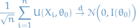
We then have,
![\begin{equation*}
\frac{1}{\sqrt{n}} \ell'(\theta_0) = \frac{1}{\sqrt{n}} \sum_{i=1}^{n} \frac{\partial}{\partial \theta} \Big[ \log f(X_i \mid \theta) \Big]_{\theta = \theta_0} = \frac{1}{\sqrt{n}} \sum_{i=1}^{n} U(X_i, \theta_0)
\end{equation*}](../../assets/latex/probability_and_statistics_8542632ebec3a8e381e6fdaf9ab23585aa75f4be.png)
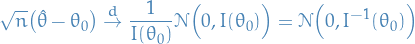
and by the Central Limit Theorem, we have
Finally, by Continuous Mapping Theorem and Slutsky's Lemma, we have
- Consistency of
Score test
For a random sample  the total score

is the sum of i.i.d. random variables. Thus, by the central limit theorem, it follows that as
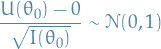
and

This can then be used as an asymptotic test of the null-hypothesis  .
.
Reject null-hypothesis if
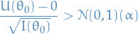
for a suitable critical value . OR equivalently,
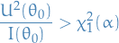
Likelihood Ratio Tests
We expand the log-likelihood using Taylor expansion about the true parameter
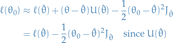
Subtracting  from both sides, and arranging
![\begin{equation*}
- 2[ \ell(\theta_0) - \ell(\hat{\theta}) ] \approx (\hat{\theta} - \theta_0)^2 J_{\hat{\theta}}
\end{equation*}](../../assets/latex/probability_and_statistics_5c7cbdd5c89c21cdc3832d688f1434cb636fe8a8.png)
And since  , we get
![\begin{equation*}
- 2[ \ell(\theta_0) - \ell(\hat{\theta}) ] \approx (\hat{\theta} - \theta_0)^2 I_{\theta_0}
\end{equation*}](../../assets/latex/probability_and_statistics_b1dbfc46182b20e94478eca536f288c872cfbccc.png)
which means that the difference between the log-likelihoods can be considered to be a random variable drawn from a  distribution
![\begin{equation*}
- 2[ \ell(\theta_0) - \ell(\hat{\theta}) ] \sim \chi^2_1
\end{equation*}](../../assets/latex/probability_and_statistics_5dbd5367f5d402842636baff39ffdb78ee7adac0.png)
and we define the term of the left side as the likelihood-ratio .
The test which rejects the  if
if
![\begin{equation*}
- 2[ \ell(\theta_0) - \ell(\hat{\theta}) ] > \chi^2_1(\alpha)
\end{equation*}](../../assets/latex/probability_and_statistics_0245a1e04db8336cd035f789881137590481e0c4.png)
for a suitable significance / critical value .
The above is just saying that we reject the null hypothesis that if the left term is not drawn from a chi-squared distribution .
Wald test
We test whether or not
That is, we reject the null-hypothesis if
for some suitable signifiance / critical value .
Generalization to multi-parameter case
Hypothesis tests
![\begin{equation*}
\begin{split}
\text{Likelihood ratio test} \quad & -2 [\ell (\boldsymbol{\theta}_0) - \ell( \hat{\boldsymbol{\theta}} )] > \chi_p^2(\alpha) \\
\text{Score test} \quad & U'(\boldsymbol{\theta}_0) I^{-1} (\boldsymbol{\theta}_0) U(\boldsymbol{\theta}_0) > \chi_p^2(\alpha) \\
\text{Wald test (ML test)} \quad & (\hat{\boldsymbol{\theta}} - \boldsymbol{\theta}_0)' I(\boldsymbol{\theta}_0) (\hat{\boldsymbol{\theta}} - \boldsymbol{\theta}_0) > \chi_p^2(\alpha)
\end{split}
\end{equation*}](../../assets/latex/probability_and_statistics_f9ff85066fe9b00b1489474d603bf6c092cc7c9e.png)
Confidence regions
![\begin{equation*}
\begin{split}
\text{Likelihood ratio} \quad & \{ \boldsymbol{\theta}: -2 [\ell(\boldsymbol{\theta}) - \ell (\hat{\boldsymbol{\theta}} ) ] < \chi_p^2(\alpha) \} \\
\text{Score} \quad & \{ \boldsymbol{\theta}: U'(\boldsymbol{\theta})I^{-1}(\boldsymbol{\theta}) U(\boldsymbol{\theta}) < \chi_p^2(\alpha) \} \\
\text{Wald (ML)} \quad & \{ \boldsymbol{\theta}: (\hat{\boldsymbol{\theta}} - \boldsymbol{\theta})' I(\boldsymbol{\theta}) (\hat{\boldsymbol{\theta}} - \boldsymbol{\theta}) \chi_p^2(\alpha) \}
\end{split}
\end{equation*}](../../assets/latex/probability_and_statistics_3fd3a827442e46511926ebf2db6f43c8ab7906b7.png)
Likelihood test for composite hypothesis
Let denote the whole parameter space (e.g.  ). In general terms we have

where  .
.
The general likelihood ratio test compares the maximum likelihood attainable if  is restricted to lie in the restricted subspace (i.e. under 'reduced' model) with maximum likelihood attainable if is unrestricted (i.e. under 'full' model):
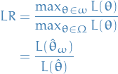
where  is the unrestricted MLE of and
  is the restricted MLE of .
Some authors define the general likelihood ratio test with the numerator and denominator swapped; but it doesn't matter.
Iterative methods

![\begin{equation*}
\boldsymbol{\theta}_{r + 1} = \boldsymbol{\theta}_r - \Bigg( \mathbb{E} \Big[ H(\boldsymbol{\theta}_r) \Big] \Bigg)^{-1} U(\boldsymbol{\theta}_r) = \boldsymbol{\theta}_r + I^{-1}(\boldsymbol{\theta}_r) U(\boldsymbol{\theta}_r)
\end{equation*}](../../assets/latex/probability_and_statistics_a0c9ffa878d32c23912bfdc09a4b75d712023ef0.png)
Simple Linear Regression (Statistical Methodology stuff)
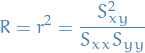
Correlation coefficient and coefficent of determination
The (Pearson) correlation coefficient is given by
and coefficient of determination
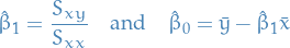
Least squares estimates
Residual sum of squares
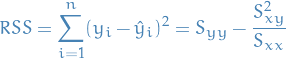
with the estimated standard deviation being

Laplace Approximation
Overview
Under certain regularity conditions, we can approximate a posterior pdf / pmf as a Normal distribution, that is
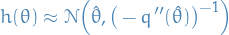
where
 i.e. the log-pdf, with
  being the second-order derivative wrt.
  is the posterior we want to approximate
"Derivation"
For any pdf that is smooth and well peaked around its point of maxima, we can use the Laplace approximation to approximate a posterior distribution by a Gaussian pdf.
It follows from taking the second-order Taylor expansion on the logarithm of the pdf.
Let denote the point of maxima of a pdf , then it also the point of maximia of the log-pdf and we can write
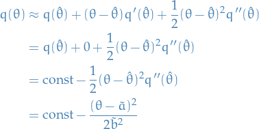
where in the second step we've used the fact that  since is a maxima, and finally let
(notice that  since is a maxima )
But the above is simply the log-pdf of a  , hence the pdf is approx. normal.
Hence, if we can find the and compute the second-order derivative of the log-pdf, we can use Laplace approximation.
Guarantees
Consider the model  ,
,  .
.
Under some regularity conditions on the pdfs/pmfs  , including all of the have the same "support", and that for each
  ,
,  is twice continuously differentiable, we have that for any prior
  which is positive, bounded and twice differentiable over
  (the parameter space),

for large .
Under the same regularity conditions it turns out that  and that
  .
.
Point estimators
Notation
- denotes a sufficient statistic
Cramér-Rao lower bound
Notation


Theorem
To state the Cramér-Rao inequality, we need to establish some regularity conditions:
 such that
  we have
  , called identifiability
 we have
  have common support
- is an open set
 exists
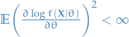
Where we remember that 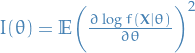 is the Fisher's information.
Let denote a random sample from and suppose that is an estimator of . Then, subject to the above regularity conditions,
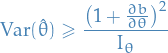
where
![\begin{equation*}
b(\theta) = \text{bias}(\hat{\theta}) \quad \text{and} \quad I_\theta = \mathbb{E} \Bigg[ \bigg( \frac{\partial \ell}{\partial \theta} \bigg)^2 \Bigg]
\end{equation*}](../../assets/latex/probability_and_statistics_2882641d26cffdddf38d341239d881241fcbbd72.png)
- For unbiased , the lower bound simplies to
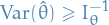
- Regularity conditions are needed to change the order of differentation and integration in the proof given below.
- Proof is for continuous r.v.s, but there is a similar proof for discrete r.v.s.
![\begin{equation*}
\begin{split}
\mathbb{E}[\hat{\theta}] &= \int \dots \int \hat{\theta}(x_1, \dots, x_n) \bigg( \prod_{i = 1}^n f(x_i \mid \theta) \bigg) \ d \mathbf{x} \\
&= \int \dots \int \hat{\theta}(x_1, \dots, x_n) L(\theta; \mathbf{x}) \ d \mathbf{x}
\end{split}
\end{equation*}](../../assets/latex/probability_and_statistics_413cfe281638ca92f751ea0c6096f1c2aea7d5f1.png)
From the definition of bias we have
![\begin{equation*}
\theta + b = \mathbb{E} [ \hat{\theta}] = \int \dots \int \hat{\theta} L(\theta; \mathbf{x}) \ d \mathbf{x}
\end{equation*}](../../assets/latex/probability_and_statistics_25bd1be1d6a6d32f84ca108253645641922184c6.png)
Differentiating both sides wrt. gives (using the regularity conditions)
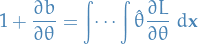
since does not depend on . Since  we have
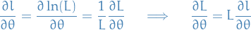
Thus,
![\begin{equation*}
1 + \frac{\partial b}{\partial \theta} = \int \dots \int \hat{\theta} \frac{\partial l}{\partial \theta} \ L \ d \mathbf{x} = \mathbb{E} \Bigg[ \hat{\theta} \frac{\partial l}{\partial \theta} \Bigg]
\end{equation*}](../../assets/latex/probability_and_statistics_274af0cfd175524bd13828d3896acee0f78d8ce4.png)
Now use the result that for any two r.v.s  and
and  ,
,

and let
Then
![\begin{equation*}
\begin{split}
\mathbb{E}[V] &= \int \dots \int \frac{\partial l}{\partial \theta} \ L \ d \mathbf{x} = \int \dots \int \frac{\partial L}{\partial \theta} \ d \mathbf{x} \\
&= \frac{\partial}{\partial \theta} \Bigg( \int \dots \int L \ d \mathbf{x} \Bigg) \quad \text{(using regularity conditions)} \\
&= \frac{\partial}{\partial \theta} 1 = 0
\end{split}
\end{equation*}](../../assets/latex/probability_and_statistics_46cfa7730829a4f18a00d645c038263a19b5e10b.png)
Hence
![\begin{equation*}
\text{Cov}(U, V) = \mathbb{E}[UV] = 1 + \frac{\partial b}{\partial \theta}
\end{equation*}](../../assets/latex/probability_and_statistics_9bf1a358b0d4be6efa0580da1e2c7c35a2374609.png)
Similiarily
![\begin{equation*}
\text{Var}(V) = \mathbb{E}[V^2] = \mathbb{E} \Bigg[ \bigg( \frac{\partial l}{\partial \theta} \bigg)^2 \Bigg] = I_\theta
\end{equation*}](../../assets/latex/probability_and_statistics_182ccac28f757f41804ad6d0040e592a6db65b35.png)
and since
we obtain the Cramér-Rao lower bound as
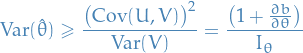
The Cramér-Rao lower bound will only be useful if it is attainable or at least nearly attainable.
Rao-Blackwell Theorem
Theorem
Let  be a random sample of observations from a distribution with p.d.f.
  . Suppose that is a sufficient statistic for and is any unbiased estimator for .
Define ![$\hat{\theta}_S = \mathbb{E}[ \hat{\theta} \mid S]$](../../assets/latex/probability_and_statistics_f67e8f86c468434c61e93025bb60d4882582973e.png) . Then,
. Then,
 is a function of only
![$\mathbb{E}[\hat{\theta}_S] = \theta$](../../assets/latex/probability_and_statistics_531c30ec2d7161de74437a71e92d7268ca95e4d2.png)

Non-parametric statistics
Maximum Mean Discrepancy (MMD)
Let be a class of functions  and let:
 be Borel probability measures
 and
and  are i.i.d. observations from and , respectively
We define the maximum mean discrepancy (MMD) as
![\begin{equation*}
\text{MMD}[ \mathcal{F}, p, q] := \sup_{f \in \mathcal{F}} \big( \mathbb{E}_x \big[ f(x) \big] - \mathbb{E}_{y} \big[ f(y) \big] \big)
\end{equation*}](../../assets/latex/probability_and_statistics_1c2a4d418cf3881d31e50de49765a5ef062d811e.png)
In the statistics literature, this is an instance of a integral probability metric.
A biased empirical estimate of the  is obtained by replacing the population expectations with empirical expectations computed on the samples and :
![\begin{equation*}
\text{MMD}_b[\mathcal{F}, X, Y] := \sup_{f \in \mathcal{F}} \bigg( \frac{1}{m} \sum_{i=1}^{m} f(x_i) - \frac{1}{n} \sum_{i=1}^{n} f(y_i) \bigg)
\end{equation*}](../../assets/latex/probability_and_statistics_d53ba6e3081c1debe50d59fce58f93002bc2518c.png)
We must therefore identify a function class that is rich enough to uniquely identify whether  , yet restrictive enough to provide useful finite sample estimates.
A RKHS is characteristic if

Wavelets
The problem with Fourier transform is that, even though we can extract the frequencies, we do not know at which time these frequencies occurr. This can be incredibly important in cases where the signal has "switches".
Idea is to
- Start with low frequency / high wavelength
- Slide over signal to extract low frequency
- Subtract high frequency away from signal
- Take higher frequency / smaller wavelength
- Slide over signal to extract higher frequency
By subtracting the low frequency we're removing the overlap of the low frequency and high frequency without interferring with the high frequency signal! Thus it's possible to extract both low and high frequencies.
A mother wavelet is some function  such that we can scale and translate to create new wavelets
  :
:
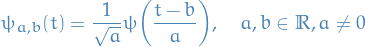
where
- is scaling
 is translation
And the Fourier transform is then
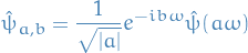
The condition required by a wavelet on  is that:
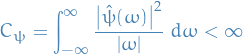
Continuous Wavelet Transform
![\begin{equation*}
W_{\psi} [f] (a, b) = \left\langle f, \psi_{a, b} \right\rangle = \int_{-\infty}^{\infty} f(t) \bar{\psi}_{a, b} (t) \ dt
\end{equation*}](../../assets/latex/probability_and_statistics_072b1d09828023553b81c052fc4af8c8fb5d6b66.png)
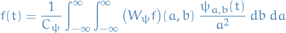
Wavelet basis
A mother wavelet is such that  form an orthogonal basis for some subspace of
  , hence
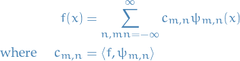
converges to in the norm!
Multi-Resolution Analysis (MRA)
- Overview
- Algorithm for constructing the different resolutions
We consider wavelets
constructed from some mother wavelet :

and we want to expand our signal in such a wavelet basis.
Consider sequence of subspaces
in
 , with the follow properties:
Nested

Union

is dense in
Orthogonality
Increased "resolution"

 such that
  is an orthogonal basis in
- is called the scaling function or father wavelet
Let
 be the "standard" scale where our mother wavelet and father wavelet live, i.e. is
  for
for  .
.
We can map
to  by
by
which is called the dilation or two-scale or refinement equation.
We can repeat this argument for arbitrary
, so with  , we write
Then,
which means
Finally, this tells us that
 (the mother wavelet) such that
constitutes an orthogonal basis for
 .
.
If
 is a multi-resolution analysis (MRA) with scaling function , then there exists a mother wavelet defined
where
which allows us to obtain an orthormal basis
for  which is dense in :
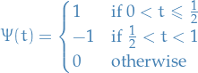
Application
For more information about how and when to apply wavelet transforms, and which mother wavelet to use, e.g., checkout MATLABs documentation on this.
Testing
Notation
 and denotes the acceptance and critical region, respectively
- denotes the critical value of some statistic

Critical region with a given significane level
is denoted
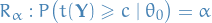
Type I error: Reject
 when is true with
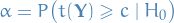
Type II error : Fail to reject
when is false (equiv., we accept when we shouldn't):
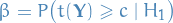
- denotes the test function:
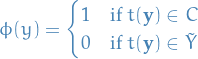
![$\mathbb{E}_{\theta} \left[ \phi(\mathbf{Y}) \right] = \mathbb{E} \left[ \phi(\mathbf{Y}) \mid \theta \right] = \mathbb{E}_{p_{\theta}} \left[ \phi(\mathbf{Y}) \right]$](../../assets/latex/probability_and_statistics_2b92c073cbdab179d6672b96fa8688a5fe0ecf71.png) refers to the expectation over whatever parametrized distribution which given you're parametrizing the distribution with .
refers to the expectation over whatever parametrized distribution which given you're parametrizing the distribution with .
Definitions
A hypothesis is simple if it defines  completely:

otherwise, it's composite.
If is parametric with more than one parameter, a composite hypothesis might specify values of some or all of them (e.g. on regression coefficient).
A U-statistic is the class of unbiased statistics; this class arise naturally in producing minimum-variance unbiased estimators (MVUEs)
Important: in statistics there are TWO notions for a U-statistic
Nonparametric statistics is the branch of statistics that is not based solely on parametrized families of probability distributions.
Thus, nonparametric tests or distribution-free tests are procedures for hypothesis testing which, unlike parametric statistics, make no assumptions about the probability distributions of the variables being assessed.
Let the data  and we wish to test two simply hypotheses:

Suppose that we choose a test statistic and reject if  for some critical value .
This induces a partition of the sample space into two disjoint regions:
the rejection region
:

the acceptance region
:

We will also sometimes use the notation  to denote the critical region which has the property
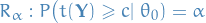
Consider and  with corresponding p.d.f.'s
  ,
,  for .
for .
For these hypotheses, comparison between the critical regions of different tests is in terms of
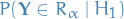
the power of a size critical region for alternative .
A best critical region is then the critical region with maximum power.
There are two possible types of error:
- Type I error: Reject when is true
- Type II error: Fail to reject when is false
- denotes the probability of Type I error and is called the significance level (or size ) of the test
 denotes the probability of Type II error which is uniquely defined only if is simple, in which case

denotes the power of the test. For composite
,  is the power function.
We can define the test function  such that
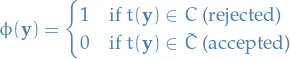
which has the property that
For discrete distributions, the probabilty that the test statistic lies on the boundary of the critical region,  , may be non-zero.
In that case, it is sometimes necessary to use a randomized test, for which the test function is
for some function  and we reject based on observed data with probability .
Suppose now there is a parametric family  of alternative p.d.f.'s for .
The power of a size critical region generalizes to the size power function
A size critical region , is then uniformly most powerful size (UMP size ) if it has maximum power uniformly over  ( is NOT power, is).
A test is UMP if all its critical regions are UMP, or more formally:
A uniformly most powerful or UMP test,  , of size is a test for which
![$\mathbb{E}_{\theta} \big[ \phi_0 (\mathbf{Y}) \big] \le \alpha, \quad \forall \theta \in \Theta_0$](../../assets/latex/probability_and_statistics_5dfdf67d44e008fef120cd0327b3d78ab866fd18.png)
Given any other test
 for which
 ![$\mathbb{E}_{\theta} \big[ \phi(\mathbf{Y}) \big] \le \alpha$](../../assets/latex/probability_and_statistics_84c4722f199becaa365cdb7e1734b2da36204336.png) for all
for all  , we have
![\begin{equation*}
\mathbb{E}_{\theta} \big[ \phi_0(\mathbf{Y}) \big] \ge \mathbb{E}_{\theta} \big[ \phi(\mathbf{Y}) \big], \quad \forall \theta \in \Theta_1
\end{equation*}](../../assets/latex/probability_and_statistics_8f438aa7ce8238487ad5d1e0f204afc7a13eca22.png)
i.e. expectation given
is at least as large as for the less powerful statistic (who's test function is ).
A test of  against
  is called unbiased of size if
![\begin{equation*}
\sup_{\theta \in \Theta_0} \mathbb{E} \left[ \phi(\mathbf{Y}) \mid \theta \right] \le \alpha
\end{equation*}](../../assets/latex/probability_and_statistics_f358da7a1208c38085dbfe718ebd698fc6466ea1.png)
and
![\begin{equation*}
\mathbb{E} \left[ \phi(\mathbf{Y}) \mid \theta \right] \ge \alpha, \quad \forall \theta \in \Theta_1
\end{equation*}](../../assets/latex/probability_and_statistics_9a79a49bf61bb7bc24f9d9a25c60f749b094d886.png)
Informally, unbiased test is one which has higher probability of rejecting when it is false, than when it is true.
A test which is uniformly most powerful among the set of all unbiased tests is called the uniformly most powerful unbiased (UMPU).
Two-sample test
The problem of comparing samples from two probability distributions, by a statistical tests of the null hypothesis that these distributions are equal against the alternative hypothesis that these distributions are different (this is called the two-sample problem), i.e. in short:
- corresponds to distributions being equal
- corresponds to distributions being different
Exact test
A test is exact if and only if
which is in contrast to non-exact tests which only have the property
for some "critical constant"  .
.
Hypothesis testing
For any size , the LR critical region is the best critical region for testing simple hypothesis vs. .
That is, suppose one is performing a hypothesis test between two simple hypothesis and  , using the likelihood-ratio test with threshold which rejects in favour of at a significance level of
where
Then,  is the most powerful test at significance level .
Bahadur efficiency
Most of this stuff is from https://www.encyclopediaofmath.org/index.php/Bahadur_efficiency.
Notation
- and denotes the null hypothesis and the alternative hypothesis
 and are the parametric set corresponding to the and , respectively
- A test statistic
 based on a random sample


 -value refers to the minimum value we require from the test for us to accept
  is the information number corresponding to
  and
and 
Stuff
- Assume large values of give evidence against
- For fixed and a real number let
Random quantity
is the value corresponding to the statistic when is the true parametric value.
For example, if
and the null hypothesis  is rejected at the significance level .
If for  with probability one we will have

then  is called the Bahadur exact slope of .
The larger the Bahadur exact slope , the faster the rate of decay of the value under the alternative. It is known that for any ,  where is the information number corresponding to and .
A test statistic is called Bahadur efficient at if
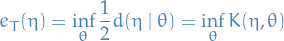
Bahadur efficiency allows one to compare two (sequences of) test statistics  and
and  from the following perspective:
Let  be the smallest sample size required to reject at the significance level on the basis of a random sample
  when is the true parametric value.
The ratio  gives a measure of relative efficiency of to .
To reduce the number of arguments, ,  and , one usually considers the rv. which is the limit of this ratio, as
  . In many situations this limit does not depend on , so it represents the efficiency of against at with the convenient formula
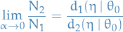
where and are the corresponding Bahadur slopes.
I.e. can use the Bahadur efficiency to compare the number of samples needed to reject .
Kolmogorov-Smirnov

 is the
 The empirical distribution function is given by
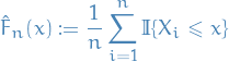
Consistency and unbiasedness at a point
Fix  , then
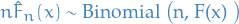
Consequently,
![\begin{equation*}
\mathbb{E} \big[ \hat{F}_n(x) \big] = \frac{1}{n} \mathbb{E} \big[ n \hat{F}_n(x) \big] = F(x)
\end{equation*}](../../assets/latex/probability_and_statistics_686c616974b5a3a767898c5ae985b63349323e0a.png)
That is,  is an unbiased estimator of for each fixed 4x$. Also
![\begin{equation*}
\text{Var}\big( \hat{F}_n(x) \big) = \frac{1}{n^2} \text{Var} \big( n \hat{F}_n(x) \big) = \frac{F(x) [1 - F(x)]}{n}
\end{equation*}](../../assets/latex/probability_and_statistics_a8ae67fb0ede2e48c804746e4caa4f3ae06a7313.png)
Consequently, by the Chebyshev inequality,
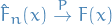
Therefore, is consistent
Kolmogorov-Smirnov test
The Kolmogorov distribution is the distribution of the rv.
![\begin{equation*}
K = \sup_{t \in [0, 1]} |B(t)|
\end{equation*}](../../assets/latex/probability_and_statistics_75ce76d3d234d22476784fb3c5a98f3340ccd722.png)
where is the Brownian bridge. The cumulative distribution function of is given by

The empirical distribution function for i.i.d. observations is defined as
![\begin{equation*}
F_n(x) = \frac{1}{n} \sum_{i = 1}^{n} I_{[- \infty, x]} (X_i)
\end{equation*}](../../assets/latex/probability_and_statistics_03be4b965828593bd5e630c5fca6943a50d56b07.png)
where
![$I_{[-\infty, x]}(X_i)$](../../assets/latex/probability_and_statistics_3dc038ff7fbccbf9dd8f92d3b652bd55aeca1992.png) is the indicatior function defined
is the indicatior function defined
![\begin{equation*}
I_{[-\infty, x]}(X_i) =
\begin{cases}
1 & \text{if } X_i \le x \\
0 & \text{otherwise}
\end{cases}
\end{equation*}](../../assets/latex/probability_and_statistics_89de4fd4d6eb8e6f7e0cf66ee19ddcf422f9b76d.png)
The Kolmogorov-Smirnov statistic for a given cumulative distribution function is
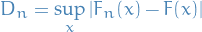
Under that the sample comes from the hypothesized distribution
![\begin{equation*}
\sqrt{n} D_n \overset{n \to \infty}{\longrightarrow} \sup_{t \in [0, 1]} | B (t) |
\end{equation*}](../../assets/latex/probability_and_statistics_208b3e9335425438be555fd5d3abd40cd5f8a1dc.png)
in distribution, where is the Brownian bridge.
If is continuous, then under  converges to the Kolmogorov distribution, which does not depend on .
Kolmogorov-Smirnov test (K-S test) is a non-parametric test of the equality of continuous , one-dimensional probability distributions that can be used to compare one sample with a reference probability distribution (one-sample K-S test ), or to compare two samples (two-sample K-S test).
The one-sample KS test is:
Using critical values of the Kolmogorov distribution, where we reject
at level if
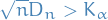
where

F-test
An F-test is any statistical test in which the test statistic, called a F-statistic, has an F-distribution under the null hypothesis.
Residual-sum of squares between two models as a F-statistic
Notation
- denotes the number of samples
- denotes the number of regressors (including the constant term)
- denotes the number of linear "restrictions" / "constraints", and therefore, also the degrees of freedom
- is
 matrix with full column rank , i.e.
  , which translates into constraints being "independent". This matrix is used to enforce the constraints on , i.e. if we don't want a constant term / intercept
  is such that
  , if the constant term was in the first entry.
  represents the hypothesized residual sum
Stuff
Consider two linear regression models with coefficients  and
and  , with
  . Then let
  and
and  denote the respective number of coefficients, with
  . Then letting
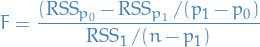
we have
i.e. the quantity above is F-distributed.
Note: observe that  so the above is a positive quantity.
Consider the null-hypothesis 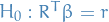 . Recall the OLS solution is given by
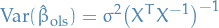
and we therefore have
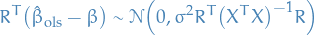
Let
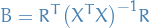
and let, using Cholesky decomposition,  be such that

we have a "matrix square root" of  in
in  . The purpose of this matrix is so we can define the following random variable:
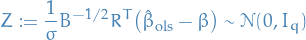
where  denotes the identity
  identity matrix. To see that this is indeed the case, observe that
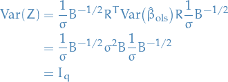
Using properties seen in the proof of 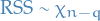 , know that this is independent of the rv.
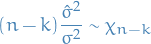
where
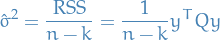
where
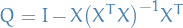
known as the residual maker matrix. Then we have
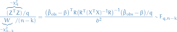
Recall that a F-statistic is a ratio between  divided by their corresponding degrees of freedom, hence the above.
In particular, under , this reduces to the statistic
divided by their corresponding degrees of freedom, hence the above.
In particular, under , this reduces to the statistic

Letting  (which is the number of components of we set to zero to get ) and
  (since this is how many parameters we now have), we conclude our proof.
Proof that 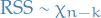
Consider the regression model

with

Then the residual vector is estimated by

And is distributed according to
and thus
![\begin{equation*}
\mathbb{E} \big[ \norm{\hat{\varepsilon}}^2 \big] = \sigma^2
\end{equation*}](../../assets/latex/probability_and_statistics_434f1a6ffdbff93d25cd1c541e8e9f3dc9066608.png)
Consider the following linear model
where  ,
,  and
and  .
The vector of residuals is estimated by
.
The vector of residuals is estimated by

where
Since trace is invariant under cyclic permutations, we have

since  matrices, and so
  . Therefore

Futhermore,
which is seen by the fact that
![\begin{equation*}
\begin{split}
Q^2 &= \Big( I - X \big( X^T X \big)^{-1} X^T \Big) \Big( I - X \big( X^T X \big)^{-1} X^T \Big) \\
&= I - X \big( X^T X \big)^{-1} X^T - X \big( X^T X \big)^{-1} X^T + \big[ X \big( X^T X \big)^{-1} \underbrace{X^T X \big( X^T X \big)^{-1}}_{= I} X^T \big] \\
&= I - 2 X \big( X^T X \big)^{-1} X^T + X \big( X^T X \big)^{-1} X^T \\
&= I- X \big( X^T X \big)^{-1} X^T \\
&= Q
\end{split}
\end{equation*}](../../assets/latex/probability_and_statistics_c7a8f5617d17a9e436e43601b88ac14a36e4171c.png)
We then have the following sequence of implications:
 only has eigenvalues
  and
and - is normal and so there exists a unitary matrix such that
Recall that

which is seen by computing ![$\mathbb{E} \big[ \big( V^T \hat{\varepsilon} \big) \big( V^T \hat{\varepsilon} \big)^T \big]$](../../assets/latex/probability_and_statistics_9b5107f237e66df714c82f29f30f146a1a27c740.png) and using
and using ![$\mathbb{E} \big[ \hat{\varepsilon} \hat{\varepsilon}^T \big] = \sigma^2 Q$](../../assets/latex/probability_and_statistics_c425ecd6c327091ca01e027fb7abd92bc8ee8e2a.png) . From this it follows that
. From this it follows that
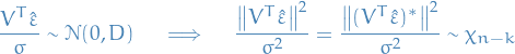
where  is the corresponding
  vector (since the rest of the components have zero variance and thus add nothing to the norm).
Furthermore, since is unitary, as mentioned earlier, we have
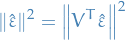
Recall that the residual sum-of-squares is given by  , and so arrive at our result
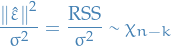
Finally, observe that this implies
Similarity testing
Notation
 with can take on values
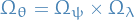
 denotes a test
Stuff
Test  vs.
vs.  .
.
is a test of size , i.e.
Then is a similar test of size .
 with
with  on the boundary of .
Confidence regions
Notation
- is drawn from some distribution


 is a size critical region for

with

- critical region refers to the sampling distribution which will lead to the rejection of the hypothesis tested when the hypothesis is true.
Stuff
- Generalization of confidence intervalls to multiple dimensions
 is a
is a  confidence region for if

If  then
then
Pivotal quantities
 which has a distribution independent of , i.e. is a pivotal statistic, that is
Then we can construct a value  such that we obtain a confidence region following:
Decision Theory
Notation
 denotes the sample space i.e.
 denotes the parameter space
 denotes a family of probability distributions
- is the action space, i.e. set of actions an experiment can take after observing data, e.g. reject or accept , estimating the value of , etc.
 denotes the loss function
 denotes decision rules , with
  is a function
  that associates a particular decision which each possible observed data set.
Stuff
For a parameter , the risk of a decision rule, , is defined as
![\begin{equation*}
R(\theta, d) = \mathbb{E}_{\theta} \Big[ \big( \theta, d(Y) \big) \Big] =
\begin{cases}
\sum_{y \in \mathcal{Y}} L \Big( \theta, d(y) \Big) f(y ; \ \theta) & \text{for discrete } \mathcal{Y} \\
\int_{\mathcal{Y}} L \Big( \theta, d(y) \Big) f(y ; \ \theta) \ dy & \text{for continuous } \mathcal{Y}
\end{cases}
\end{equation*}](../../assets/latex/probability_and_statistics_b77811a2c9f897a2cf753569e3d6d72260fb7031.png)
In other words, the risk is the expected loss of a particular decision rule when the true value of the unknown parameter is .
Note: this is fundamentally a frequentist concept, since the definition implicitly invokes the idea of repeated samples from the parameter space and computes the average loss over these hypothetical repetitions.
Selection of decision rule
Given two possible decision rules and , the rule strictly dominates the rule if

and there exists at least one value of , e.g. θ', for which
It is clear that we would always prefer to .
If, for a given decision rule , there exists some decision rule that strictly dominates , then is said to be inadmissible.
Conversely, if there is no decision rule that dominates , then is said to be admissible.
That is, generally less-than-or-equally AND has at least ONE value of for which we have strict inequality.
Unbiasedness
We say a loss-function is unbiased if
![\begin{equation*}
\mathbb{E}_{\theta} \Big[ L \big( \theta', d(Y) \big) \Big] \ge \mathbb{E}_{\theta} \Big[ L(\theta, d(Y) \Big], \quad \forall \theta, \theta' \in \Omega_{\theta}
\end{equation*}](../../assets/latex/probability_and_statistics_1e495084263dfd7cac89cd62e28f348850ddb2c9.png)
i.e. loss of the decision rule should be minimized for the true value of the parameter .
Minimax decision rules
A decision rule is minimax if it minimizes the maximum risk

which can also be written
Bayes decision rules
The Bayes risk of a decision rule, , is defined by
or by a sum in case of discrete-valued probability distribution.
A decision rule is a Bayes rule with respect to the prior  if it minimizes the Bayes risk, i.e.,
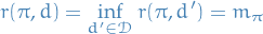
Definition of Bayes risk assumes that the infimum is achieved by some rule, which might not always be true.
In those cases, for any , we can find a decision rule  such that
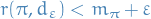
Such a rule is said to be  *Bayes wrt. prior .
A useful choice of prior is the one that is most conservative in its estimate of risk. This gives rise to the concept of a least favourable prior.
We say  is a least favourable prior if, for any other prior
  we have
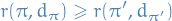
where  are the Bayes (decision) rules corresponding to and
  .
.
Randomized decision rules
- decision rules
 which we choose from with probabilties
  , with
  and
and 
Define
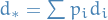 to be the rule "selection decision rule
  with prob.
  ", called the randomized decision rule, which has risk
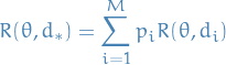
- Sort of a linear combination of decision rules
- Minimax rules are often this way
- Supremum over of the risk for
 is smaller than the supremum of the risk for any of the decision rules individually
- Supremum over
Finding minimax rules
Suppose that  is a Bayes (decision) rule corresponding to prior
  and
and  , then
- is a minimax decision rule
- is the least favourable prior
Admissibility of Bayes (decision) rules
We have the following three theorems:
Assume that the parameter space,  , is finite and a given prior gives positive weight to each
  .
.
The a Bayes (decision) rule wrt. is admissible.
If a Bayes (decision) rule is unique, it is admissible.
Let be a subset of the real line. Assume that hte risk functions  are continuous in for all decision rules .
If the prior has the property that for any and any , the interval  has non-zero probability under , then the Bayes (decision) rule wrt. is admissible.
James-Stein Estimators
Notation

 is the square loss function
Risk of a decision rule is then given
![\begin{equation*}
R\Big( \mu, \hat{\mathbf{d}}^0(\mathbf{Y}) \Big) = \mathbb{E} \Big[ \norm{\mu - \mathbf{Y}} \Big]^2 = \sum_{i=1}^{p} \mathbb{E} \big[ (\mu_i - Y_i)^2 \big] = \sum_{i=1}^{p} \text{Var}(Y_i)
\end{equation*}](../../assets/latex/probability_and_statistics_2e8525d65e4bb539bb0116945f5781cc319156b9.png)
Stein's Paradox
The class of James-Stein estimators of the form
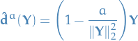
has smaller risks that are also independent of and hence strictly dominate the natural estimator

These are called shrinkage estimators as they shrink towards when  , and has the following consequence: folding in information from variables that are independent of the variable of interest can, on average, improve estimation of the variable of interest!
Suppose
and  is an almost differentiable function then
![\begin{equation*}
\frac{1}{\sigma^2} \mathbb{E} \Big[ (\mathbf{X} - \mu) f(\mathbf{X}) \Big] = \mathbb{E} \Big[ \nabla f(\mathbf{X}) \Big]
\end{equation*}](../../assets/latex/probability_and_statistics_9d084ea14dd7bf28bc5e8f5258a63c239033506e.png)
First we do the univariate case.
Suppose
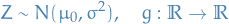
which is absolutely continuous, and
![\begin{equation*}
\mathbb{E} \big[ g'(Z) \big] < \infty
\end{equation*}](../../assets/latex/probability_and_statistics_54d8dd82c3a81f88ffe111bfa400c5e1542d061c.png)
Using change of variables to set  and
and  , then is std. normal. Then
Then one simply substitute into the Stein's lemma and prove that it is indeed satisfied.
Bayesian Statistics
Model comparison
Bayesian Information Criterion (BIC)
Bayesian Information Criterion (BIC) is a criterion for model selection among a finite set of models; the model with the lowest BIC is preferred.
The BIC is defined as:

where
 is the MLE of the model
- the obsered data
- is the number of data points in
- is the number of parameters in the model
BIC is an asymptotic result derived under the assumptions that the data distribution follows an exponential family.
Limitations:
- Approximation only valid for sample sizes

- The BIC cannot handle complex collections of models as in the variable selection problem in high-dimensions
Akaike Information Criterion (AIC)
- Given collection of models for some data, estimates quality of each model, relative to each of the other models
- NOT a test of model in a sense of testing a null hypothesis, i.e. says nothing about the absolute quality, only relative quality
Suppose we have a statistical model of some data.
Let:
- be the number of estimated parameters in the model
- be the maximum value of the likelihood function for the model
Then the Akaike Information Criterion (AIC) value of the model is

Given a set of candidate models for the data, the preferred model is the one with the minimum AIC value.
Thus, AIC rewards goodness-of-fit (as assessed by the likelihood function), but it also penalizes large number of parmateres (complexity).
AIC is based on information theory. Suppose data was generated by some unknown process , and we're considering two candidate models to  and
and  . We could then compute the KL-divergence of and ,
  , and of and ,
  , i.e. the "loss of information" by representing using or , respectively. One could then compare these values, and choose the candidate model which had the smallest KL-divergence with .
Asymptotically, making this choice is equivalent of choosing the model  with the smallest
AIC! Note, however, that AIC can be a bad comparison if the number of samples is small.
TODO ANOVA
One-way
Two-way
Bootstrapping
- Bootstrap methods gets its name due to "using data to generate more data" seems analogous to a trick used by the fictional Baron Munchausen, who when he found himself at the bottom of a lake got out by pulling himself up by his bootstraps :)
Notation
 is a single homogenous sample of data with PDF and CDF
 - Statistic whose value in the sample is , which estimates , an underlying characterstic of the population. Generally is a symmetric function of
- EDF stands for the empirical distribution function, denoted

 denotes the parameter of a parametric model with CDF and PDF
  and
and  , respectively
 is the fitted model to data drawn from the PDF
  denotes the rv. distributed according to the fitted model, and we do the same for other moments (e.g.
  denotes the mean of the fitted model)
 denotes the random variable of the statistic of interested, in comparison to which is the observed estimate, or rather

Stuff
- Interested in probability distribution of
 describes the fact that the population parameter is equal to the value the statistic takes on for the underlying CDF
  expresses the relationship between the estimate and
- To be properly rigorous, we would write
 and require that
  as , possibly even that
- We will mostly assume

- To be properly rigorous, we would write
Moment estimates
- Suppose we simulate a dataset
 , i.e. from fitted model
 - Properties of
 are then estimated from
  , using repetitions of the data simulation
 - Important to recognize that we are not estimating absolute properties of , but rather of relative to
Distribution and quantile estimates
- Approximating the distribution of by that of

Cumulative probabilities are estimated by EDF of the simulated values
 , i.e. if
then the simulation estimate of
 is
is
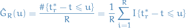
And
 , the exact CDF of under sampling from the fitted model
- Approximation
 to
to  contains two sources of error:
 to due to data variability
- to due to finite simulation
- Quantiles of distribution of
- Approximated using ordered values of
Suppose
 are independent distribution with CDF and if
  denotes the j-th ordered value, then
![\begin{equation*}
\mathbb{E} \big[ X_{(j)} \big] = K^{-1} \bigg( \frac{j}{N + 1} \bigg)
\end{equation*}](../../assets/latex/probability_and_statistics_eafdc619839199c74413ce20a1ca0690dbedbf83.png)
- This implies a sensible estimate of
 is the
  , assuming that
  is an integer
- Therefore we can estimate quantile of by the
 oredered value of , i.e.
- We're assuming is chosen so that
 is an integer
- Therefore we can estimate
- Approximated using ordered values of
Nonparametric simulation
- Same as in previous section, but EDF to perform simulation instead of estimate of parameter for distribution (e.g. using MLE estimate of ); call this nonparametric bootstrap
Simple confidence intervals
If we use bootstrap estimates of quantiles for , then an equitailed  confidence interval will have limits
where we explicitly write the second term in the parenthesis in the limits to emphasize that we're looking at with an expectation .
This is based on the probability implication

Reducing error
- Problem: choose quantity
 such that is as nearly pivotal as possible
- That is, it has (at least approx.) the same distribution under sampling from both and
- That is, it has (at least approx.) the same distribution under sampling from both
Let
 with
with  increasing in and if
  is an approx. lower quantile of
  , then

where
 is the inverse transformation
- Thus,
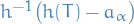 is an upper confidence limit for
So we're basically saying "Let's bound the difference between of the true and of our estimator by , with a certainty / probability of  "
"
OR rather, "let's bound the probability of the difference between and  being "
OR "we want some constant such that the probability of and differ by more than to be bounded by ", and we
Theoretical basis for bootstrap
Suppose we have a random sample , or equiv., its EDF .
We want to estimate some quantity 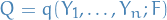 , e.g.
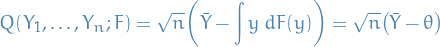
and want to estimate the distribution function

where the conditioning on indicates that is a random sample from .
The bootstrap estimate of  is then

where in this case

In order for
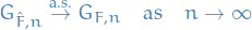
we need the following conditions to hold (letting be a neighborhood of in a space of suitable distributions):
- For any
 ,
,  must converge weakly to a limit
- This convergence must be uniform on
- The function mapping to
 must be continuous
where converge weakly means
for all integrable functions  .
.
Under these conditions, the bootstrap estimate is consistent.
Resampling for testing
Nonparametric Permutation tests
- Permutation test is a two-sample test
- Have samples
 and
and  for two distributions.
 - Want to check if
 is true
 Consider some statistic which measure discrepancy between the two sample-sets, e.g. mean difference

- Under , for every sample
 , whether or not the sample came from distribution or should be equally likely, since under we have
 - Therefore we consider consider permutations between the samples form the distributions!
Consider
 tuple
tuple

Permute the tuple

where
is a permutation on symbols.
- Let
 and
and 
- Compute assuming
 to come from and
  to come from .
Gives us achieved significance level (ASL), also known as the p-value, by considering
i.e. the probability of getting a
large value when is true
- Observe that is a "discrepancy" measurement between the samples, e.g. the difference, and so "large values = BAD"
- Observe that
Practically, there can be a lot of permutations to compute;  possibilities, in fact. Therefore we estimate the
  by "sampling" permutations uniformly:
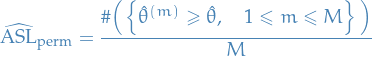
where  corresponds to the estimate of using the m-th sampled permutated dataset, and is the number of permutations considered.
Note: permutation test is an exact test when all permutations are computed.
Frequentist bootstrapping
- Data approximates unknown distribution
- Sampling distribution of a statistic can be approximated by repeatedly resampling the observations with replacement and computing the statistic for each sample
Let
 denote the original samples
 denote the bootstrap sample
- Likely have some observations repeated one or more times, while some are absent
Equivalently, we can instead make the following observation:
- Each original observation
 occurs anywhere from to times
 Let
 denote # of times occurs in
  and
and
thus
Let
 such that
then
- Hence we can compute the bootstrap sample by instead drawing
 this way, and weighting the original samples by these drawn weights!
Recall that
has the property that

Hence,
TODO Bayesian bootstrapping
Problems / Examples
Multi-parameter MLE
Normal samples
Suppose we have the samples  following the model
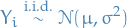
Then we want to test  against
  .
.
The likelihood is given by
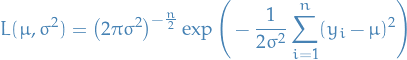
Under our restricted parameter-space (): then the MLE
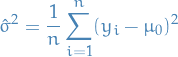
Under  (
( and can take on any value):
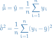
Thus, the likelihood ratio is
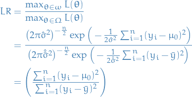
But
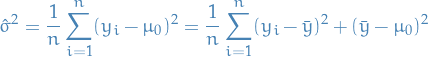
and thus
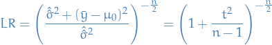
where
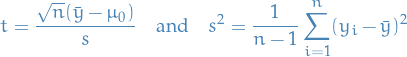
Rejecting for small values for LR is equivalent to rejecting for large values of  , i.e. this test is equivalent to a two-tailed t-test.
Here we can determine an exact distribution for LR, or rather the equivalent test statistics , i.e.

However, in general, the distribution of LR (under ) is difficult to determine and we need to use the approximate method.
Fisher's method of scoring
Multiparameter case
Let be i.i.d. with
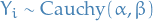
with p.d.f.
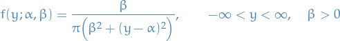
that is  .
.
Log-likelihood:
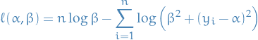
Score vector:
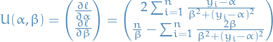
Hessian matrix:
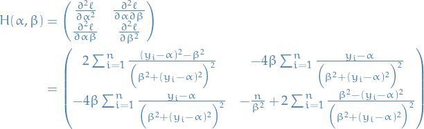
Observed information matrix:
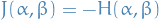
Expected information matrix:
![\begin{equation*}
I(\alpha, \beta) = - \mathbb{E}[H(\alpha, \beta)] = \frac{n}{2 \beta^2} \begin{pmatrix}
1 & 0 \\
0 & 1
\end{pmatrix}
\end{equation*}](../../assets/latex/probability_and_statistics_a7a6320450411e834e2766e9352c5b500bc8579b.png)
Asymptotic variance-covariance matrix of
is:
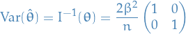
Estimated standard errors:
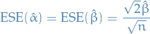
Covariance between our estimates:
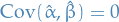
Asymptotic distribution:
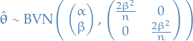
Which is the distribution we would base a Wald test of
 on, i.e.
Asymptotics
Overview
- A lot of it based on van2000asymptotic
Notation
For a measure
on a measurable space  and a measurable function
  ,
,

 denotes the empirical measure, such that
 denotes the empirical process, i.e. the "cenetered & scaled" version of ,
![\begin{equation*}
\mathbb{G}_n f = \sqrt{n} \big( \mathbb{P}_n f - Pf \big) = \frac{1}{\sqrt{n}} \sum_{i=1}^{n} \big( f(X_i) - \mathbb{E}_p [ f(X_i) ] \big)
\end{equation*}](../../assets/latex/probability_and_statistics_0a81db4efc68ca9ee36cce132512331704d0f806.png)
 denotes a P-Brownian bridge
 denotes the upper α-quantie of a std. normal
 denotes the upper α-quantie of a χ²-distribution
 denotes the upper α-quantie of a t-distribution
 denotes absolutely continuous
 denotes contiguous
 denotes mutually contiguous
 denotes weak convergence, and if has distribution , we also write
For a given sequence of random variables

where
 denotes the fact that a sequence is bounded in probability.
Stochastic convergence
For any random vectors  and the following statements are equivalent
 for all continuity points of
![$\mathbb{E} [f(X_n)] \to \mathbb{E}[f(X)]$](../../assets/latex/probability_and_statistics_e3aad164dab5cf25ef60f779a7acf1b5f440b7fa.png) for all bounded, continuous functions , i.e.
for all bounded, continuous functions , i.e. 
- for all bounded, Lipschitz functions
![$\liminf \mathbb{E}[f(X_n)] \ge \mathbb{E}[f(X)]$](../../assets/latex/probability_and_statistics_3eb0d92d6baec89d54582e97d1e0437e702ad17d.png) for all nonnegative, continuous functions
for all nonnegative, continuous functions  for every open set
  for every closed set
  for all Borel sets with
  , where
  is the boundary of
lemma:portmanteau-weak-convergence-equivalences is a very useful lemma for talking about convergences in
Any random vector is tight : for every

A set of random vectors  is called uniformly tight if can be chosen the same for every
  : for every

Thus, there exists a compact set to which all give probability "almost" one.
Another name of uniformly tight is bounded in probability.
Let be random vectors in  .
.
- If for some , then
 is uniformly tight.
 - If is uniformly tight, then there exists a subsequence with
 as
as  for some .
Prohorov's theorem states that every uniformly tight sequence contains a weakly converging subsequence. This basically generalizes the Heine-Borel theorem to random vectors.
Characteristic functions
Let and be random vectors in . Then
![\begin{equation*}
X_n \leadsto X \quad \iff \quad \mathbb{E} \big[ e^{i t^T x_n} \big] \to \mathbb{E} \big[ e^{i t^T X} \big], \quad \forall t \in \mathbb{R}^k
\end{equation*}](../../assets/latex/probability_and_statistics_676407f91683756d1605ffde81c570712b706c97.png)
Moreover, if ![$\mathbb{E} \big[ e^{it^T X_n} \big]$](../../assets/latex/probability_and_statistics_09f0e4437758136600aa4be8668f990335e5a939.png) convergences pointwise to a function
convergences pointwise to a function  that is continuous at zero, then is the characteristic function of a random vector and .
Statistical Learning Theory
Notation
Binary classification
Notation
 denotes the training data for the algorithm
 and
and  for convenience
 denotes the class of binary classifiers considered, and thus
Symmetrization
- Idea: replace the true risk
 by an estimate computed on an independent set of data, i.e.
  (called a virtual or ghost sample)
For any .s.t that  ,
,
![\begin{equation*}
\Pr \bigg[ \sup_{f \in \mathcal{F}} \big( P - P_n \big)f \ge t \bigg] \le 2 \Pr \bigg[ \sup_{f \in \mathcal{F}} \big( P_n' - P_n \big)f \ge t / 2 \bigg]
\end{equation*}](../../assets/latex/probability_and_statistics_2e47076fbc441cd4ab0390a9cc753c4f38bcc02b.png)
where
 denotes the empirical measure of the "ghost" sample
Stuff
For a class of functions, the Rademacher average is defined as
![\begin{equation*}
\mathcal{R}(\mathcal{F}) = \mathbb{E} \Big[ \sup_{f \in \mathcal{F}} R_n f \Big]
\end{equation*}](../../assets/latex/probability_and_statistics_606bb8834f77d4808279fe9419d8f22420fb0d4a.png)
where
 is defined
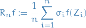
 are Rademacher random variables, i.e. i.i.d. such that
  .
. denotes the expectation over all the rvs, i.e.
Similarily, the conditional Rademacher average is defined as
![\begin{equation*}
\mathcal{R}_n(\mathcal{F}) := \mathbb{E}_{\sigma} \Big[ \sup_{f \in \mathcal{F}} R_n f \Big]
\end{equation*}](../../assets/latex/probability_and_statistics_abbe3201f982b43430093f75f0b1b6414ea61623.png)
where
 denotes the expectation only over the rvs
  , conditioned on
For all  , with probability at least
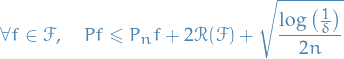
and also, with prob. at least ,
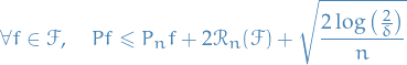
where
True risk
![\begin{equation*}
Pf := \mathbb{E} \big[ f(X, Y) \big]
\end{equation*}](../../assets/latex/probability_and_statistics_bd938671795fdb30032bec6ae59f9a6b0d25a59d.png)
Empirical risk
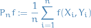
Topics in Statistical Theory
1.2 Estimating an arbitrary distribution function
Let
 denote the class of all dsitribution functions on
Empirical distribution
 is given by
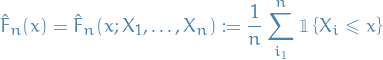
We have
as .
Given , let  .
.
Set  , and
, and
and  .
.
Writing  , which we can do since is left-continuous, we note that
Let
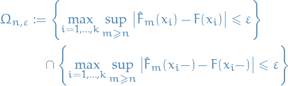
where
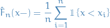
(note the that this has uses strict inequality). Hence, by a union bound, we have
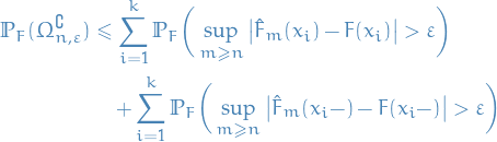
which, by SLLN the terms in the absolute values goes to zero a.s. as  , therefore implying that
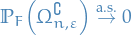
Now fix and find  s.t.
s.t.  . Then for any
  and
and  ,
,
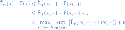
where in the second inequality we use the fact that  .
.
Similarily, for the other way around, we have
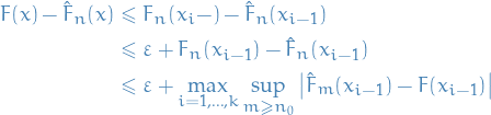
From the two equations above, it follows that
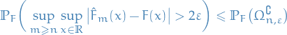
since either we have
 : in which case the event on the LHS can occur if
 : in which case the event on the LHS can occur if
 1
1
Hence the probability of such an event is upper-bounded by the RHS  .
.
We therefore conclude that
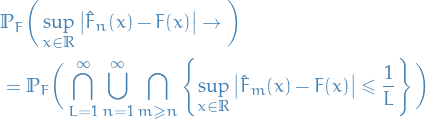
i.e. for all  ,
,  such that
  , the difference is less than
  .
.
In particular, note that the probability on the RHS is:
- Decreasing in (since the event becomes smaller as increases)
- Increasing in (since the "number of"
 we're taking the intersection for decreases)
This means that we have
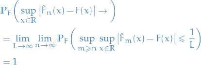
as we wanted.
1.3
Let
 be a sequence of random vectors in
Suppose  and a random vector such that
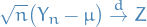
as .
Furthermore, suppose that  is differentabile at .
Then
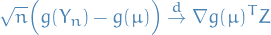
This can be seen by using expanding using the Taylor expansion at .
1.4. Concentraion Inequalities
We say the random variable is sub-Gaussian with parameter if and it has MGF
![\begin{equation*}
\mathbb{E} \big[ e^{tX} \big] \le e^{t^2 \sigma^2 / 2}, \quad \forall t \in \mathbb{R}
\end{equation*}](../../assets/latex/probability_and_statistics_3c5fed34a5a24bc4a09dd636e33331db17ddf3af.png)
For any  , we have
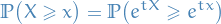
By Markov's inequality we have
![\begin{equation*}
\begin{split}
\mathbb{P} \big( X \ge x \big) &\le \frac{\mathbb{E} \big[ e^{tX} \big]}{e^{t x}} \\
&\le e^{- tx} e^{t^2 \sigma^2 / 2}
\end{split}
\end{equation*}](../../assets/latex/probability_and_statistics_afba67577dddf6d382535edd3322ebf9ac549984.png)
where in the second inequality we used the fact that is sub-Gaussian with parameter . Since this holds for any  ,
,
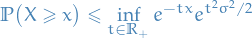
The RHS attains the minimum at  (this can be seen by expanding the square and the solving the resulting quadratic), thus
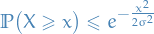
as claimed!
Let be independent r.v.s. with
![$\mathbb{E} [X_i] = 0$](../../assets/latex/probability_and_statistics_0be76112efe56b9d813f5c9b0b78863d116153ec.png)
- finite variances
 for some
Moreover, let

 defined by
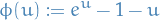
Then, for every  ,
,
![\begin{equation*}
\log \mathbb{E} \big[ e^{t S} \big] \le \frac{n \nu}{b^2} \phi(b t)
\end{equation*}](../../assets/latex/probability_and_statistics_c5369980d547464e6c9ea0a741d8e6d7bc0bc90e.png)
Consequently, defining
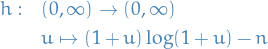
we have that for ,
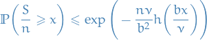
Define
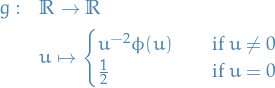
where the definition at  , is simply to ensure continuity for all
  .
.
Then is icnreasing, so for ,
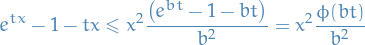
Hence, for ,
![\begin{equation*}
\begin{split}
\log \mathbb{E} \big[ e^{t S} \big] &= \sum_{i = 1}^{n} \log \mathbb{E} \big[ e^{t X_i} \big] \\
&\le \sum_{i = 1}^{n} \log \bigg( 1 + \mathbb{E}\big[ X_i^2 \big] \frac{\phi(bt)}{b^2} \bigg) \\
&\le n \log \bigg( 1 + \frac{\nu \phi(bt)}{b^2} \bigg) \\
&\le n \frac{\nu \phi(bt)}{b^2}
\end{split}
\end{equation*}](../../assets/latex/probability_and_statistics_3fd7d9524ee3bb240d57fee17a0e2c1b38e5780c.png)
where in the
- second to last inequality we have multiplied by
 and used Jensen's inequality,
 - final inequality we used the fact that
 for
for  .
.
Consequently, by a Chernouff bound,
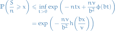
since the infimum is attained at 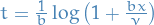 .
.
Bibliography
Bibliography
- [arjovsky17_wasser_gan] Arjovsky, Chintala, Bottou & L\'eon, Wasserstein Gan, CoRR, (2017). link.
- [roberts04_gener_state_space_markov_chain_mcmc_algor] Roberts & Rosenthal, General State Space Markov Chains and Mcmc Algorithms, CoRR, (2004). link.
- [gelman2013bayesian] Gelman, Carlin, Stern, Dunson, Vehtari & Rubin, Bayesian data analysis, Chapman and Hall/CRC (2013).
- [adrian13_count_model_based_weibul_inter_times] Adrian, Bradlow, Fader, & McShane, Count Models Based on Weibull Interarrival Times, CoRR, (2013). link.
- [yannaros1994weibull] Yannaros, Weibull renewal processes, Annals of the Institute of Statistical Mathematics, 46(4), 641-648 (1994).
- [clauset07_power_law_distr_empir_data] Clauset, Shalizi, & Newman, Power-Law Distributions in Empirical Data, CoRR, (2007). link.
- [so_you_think_you_have_a_power_law_shalizi] Cosma Shalizi, So You Think You Have a Power Law - Well Isn't That Special?, link.. (Accessed on 05/22/2018)
- [likelihood_ratio_test_for_model_selection_and_non_nested_hypothesis_vyong89] Quang Vuong, Likelihood Ratio Tests for Model Selection and Non-Nested Hypotheses, Econometrica, 57(2), 307-333 (1989). link.
- [van2000asymptotic] Van der Vaart, Asymptotic statistics, Cambridge university press (2000).