Algebra
Table of Contents
Notation
 denotes a group
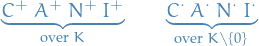
- CANI stands for:
- Commutative
- Associative
- Neutral element (e.g. 0 for addition)
- Inverse
Terminology
- almost all
- is an abbreviation meaning "all but finitely many"
Definitions
Homomorphisms
A homomorphism  is a structure-preserving map between the groups and
  , i.e.

A endomorphism is a homomorphism from the group to itself, i.e. 
 .
.

Linear isomorphism
Two vector spaces  and
and  are said to be isomorphic if and only if there exists a linear bijection
  .
.
Field
An (algebraic) field  is a set
  and the maps


that satisfy
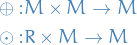
Vector space
A vector space  over a field
  is a pair consisting of an abelian group
  and a mapping

such that for all  and
and  we have A D D U:
- Associativity:

- Distributivity over field-addition:

- Distributivity over field-multiplication:

- Uint:

Ring
 over a set
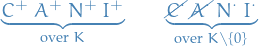
Equivalence relations
A equivalence relation on some set is defined as some relation betweeen  and
and  , denoted
  , such that the relation is:
- reflexive:

- symmetric:

- transistive

Why do we care about these?
- Partitions the set it's defined on into unique and disjoint subsets
Unitary transformations
A unitary transformation is a transformation which preserves the inner product.
More precisely, a unitary transformation is an isomorphism between two Hilbert spaces.
Groups
Notation
![$[G : H]$](../../assets/latex/algebra_113a390f333ef98f5d83a6bd467913647b2d6881.png) or
or  denotes the number of left cosets of a subgroupd of , and is called the index
Definitions
The symmetric group  of a finite set of
  symbols is the group whose elements are all the permutation operations that can be performed on the distinct symbols, and whose group operation is the composition of such permutation operations, which are defined as bijective functions from the set of symbols to itself.
An action of a group is a formal way of interpreting the manner in which the elements of the group correspond to transformations of some space in a way that preserves the structure of the space.
If is a group and  is a set, then a (left) group action
  of on is a function
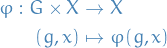
that satisfies the following two axioms (where we denote  as
as  ):
):
- identity:
 for all
  (
( denotes the identity element of )
 - compatibility:
 for all
  and all
where  denotes the result of first applying
  to
to  and then applying
  to the result.
From these two axioms, it follows that for every  , the function which maps to
  is a bijective map from to . Therefore, one may alternatively define a group action of on as a group homomorphism from into the symmetric group
  of all bijections from to .
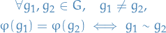
The action of on is called transistive if is non-empty and if:

Faithful (or effective ) if

That is, in a faithful group action, different elements of induce different permutations of .
In algebraic terms, a group acts faithfully on if and only if the corresponding homomorphism to the symmetric group,  , has a trivial kernel.
If does not act faithfully on , one can easily modify the group to obtain a faithful action. If we define:

then  is the normal subgroup of ; indeed, it is the kernel of the homomorphism . The factor group
  acts faithfully on by setting
  .
.
We say a group action is free (or semiregular or fixed point free ) if, given ,

We say a group action is regular if and only if it's both transitive and free; that is equivalent to saying that for every two  there exists precisely one s.t.
  .
.
Consider a group acting on a set . The orbit of an element in is the set of elements in to which can be moved by the elements of . The orbit of is denoted by  :
:

An abelian group, or commutative group, is simply a group where the group operation is commutative!
A monoid is an algebraic structure with a single associative binary operation and an identity element, i.e. it's a semi-group with a binary operation.
Cosets
Let be a group and be a subgroup of . Let . The set

of products of with elements of , with on the left is called a left coset of in .
The number of left cosets of a subgroup of is the index of in and is denoted by  or . That is,
![\begin{equation*}
[G : H] = \left| G / H \right|
\end{equation*}](../../assets/latex/algebra_b04fe081606903544e6cfd4f4c4eda2f4b142fe8.png)
Center
Given a group , the center of , denoted  is defined as the set of elements which commute with every element of the group, i.e.

We say that a subgroup of is central if it lies inside , i.e.  .
.
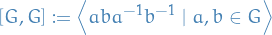
Abelianisation
Given a group , define a abelianisation of to be the quotient group

with  is the normal subgroup generated by the commutators
  for
for  , i.e.
Theorems
Let be a group of order and let  be a prime divison of .
Then has an element of order .
Fermat's Little Theorem
Let be a prime number.
Then for  , the number
  is an integer multiple of . That is

Isomorphism theorems
Let
- be a group homomorphism
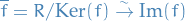
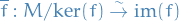
Then  is a normal subgroup of , and
  . Furthermore, there is an isomorphim
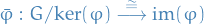
In particular, if is surjective, then

Le be a group,  and
and  .
.


First
 so clearly
  .
Let
.
Let  and
and  . We then want to show that
  .
Observe that
.
Observe that

since
 .
So
.
So  so that
 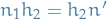 ,
,
And now we check that the

Let
 ,
,  . Wan to show that
  .
.
- Let
 ,
,  . Then
  since , so , for all .
 Want to show that
 .
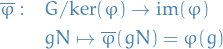
First Isomorphism Theorem tells us that
.
First Isomorphism Theorem tells us that

Therefore, letting

where we simply factor out the
from every element in  .
.

So
maps into  , but we need it to be surjective, i.e.

An element of
is a coset  for
for  , which is clearly
  . And finally,
Hence, by the First Isomorphism Theorem,

Notice  . In fact,
  .
.
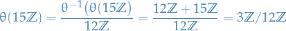
As an example,  . Then

by the First Isomorphism Theorem and since  .
And, we can also write
.
And, we can also write
since  .
.
Want to show that both are isom. to  . We do this by constructing map:
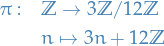
and just take the coset. And,

Hence by 1st Isom. Thm.

Kernels and Normal subgroups
Arising from an action  of a group on a set , is the homomorphism

the permutation of corresponding to .
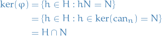
The kernel of this homomorphism is also called the kernel of the action and is denoted  .
.
Remember,

is the permutation  . Therefore,
  if and only if
  for all , and so

consists of those elements which stabilize every element of .
Let be a subgroup of a group , and let  .
.
The conjugate of by , written  , is the set

of all conjugate of elements of by .
This is the image  of under the conjugation homomorphism
  where
where  .
.
Hence, is a subgroup of .
Let be a subgroup of .
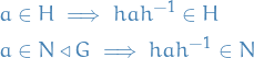
If  for all , then

A subgroup of a group, , is called a normal subgroup if it is invariant under conjugation; that is, the conjugation of an element of by an element of is still in :

 . Then
  if and only if
  for all .
Let and be groups.
The kernel of any homomorphism  is normal in .
Hence, the kernel of any group action of is normal in .
Let be a group acting on the set  of left cosets of a subgroup of .
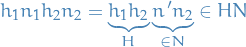
- The stabilizer of each left coset
 is the conjugate
- If
 for all then
Factor / Quotient groups
Let be a group acting on a set and be the kernel of the action.
The set of cosets of in is a group with binary operation

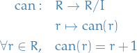
which defines the factor group or quotient group of by and is denoted

But I find the following way of defining a quotient group more "understandable":
Let  be a group homomorphism such that
That is, maps all distinct  which are equivalent under
  to the same element in
  , but still preserves the group structure by being a homomorphism of groups.
There is a function  with
with

For we have that

thus  is a homomorphism.
Then, clearly

is called the natural homomorphism from to .

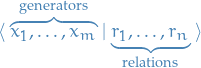
Group presentations
Notation
 or
or  refers to the group generated by such that
 denote is the free group as generated by
 In general:
 , e.g.
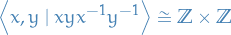
where the "unit-condition" simply specifies that the group is commutative
Free groups
 is the free group generated by
  .
.
Elements are symbols in  , subject to
- group axioms
- " and all logical consequences :) "
Let  .
.
The group with presentation
is the group generated by subject to
- group axioms

- " and all logical consequences :) "
There's no algorithm for deciding whether  is the trivial group.
Let  and let
  , where is a group.
Then there is a unique homomorphism:
And the image of  is the subgroup of generated by
  .
.
Central Extensions of Groups
Let
 be an abelian group
- be an arbitrary group
An extension of by the group is given an exact sequence of group homomorphisms

The extension is called central if is abelian and its image  , where
  denotes the center of
  , i.e.

For a group acting on another group by a homomorphism  , the semi-direct product group
  is the set
  with the multiplication given by the formula

This is a special case of a group extension with  and
and  :
:

Exact sequence
An exact sequence of groups is given by

of groups and group homomorphisms, where exact refers to the fact that

Linear Algebra
Notation
 denotes the set of all matrices on the field
 ![$M_\mathcal{B}^\mathcal{A} = {}_\mathcal{B}[f]_\mathcal{A}$](../../assets/latex/algebra_1a3e01cd9b152a4a99ee466373fc7699987ae513.png) denotes the representing matrix of the mapping
denotes the representing matrix of the mapping  wrt. bases
  and
and  , where is ordered basis for and ordered basis for
  :
:
![\begin{equation*}
{}_\mathcal{B}[f]_\mathcal{A} = {}_\mathcal{B}[f]_{\mathcal{B}} \circ {}_{\mathcal{B}}\text{id}_{\mathcal{A}} \circ {}_\mathcal{A}[f]_\mathcal{A}
\end{equation*}](../../assets/latex/algebra_4e130107b602d6cee146ac936051ccb2fb027981.png)
![${}_\mathcal{B}[f] = {}_{\mathcal{B}}\text{id} [f]$](../../assets/latex/algebra_0523db315c405d3dbc83dcb0ab9de97b988670c7.png) and
and ![$[f]_{\mathcal{B}} = [f] \text{id}_{\mathcal{B}}$](../../assets/latex/algebra_9b4615d88f6ccbc4460b13a1862bb2f7f32c8e1f.png) where
where  denotes the "identity-mapping" from elements represented in the basis to the representation in .
 denotes the n-dimensional standard basis
 , i.e. the set of non-zero elements of
Vector Spaces
Notation
- is a set
- is a field


Basis
A subset of a vector space is called a generating set of the vector space if its span is all of the vector space.
A vector space that has a finite generating set is said to be finitely generated.
 is called linearly independent if for all pairwise different vectors
  and arbitrary scalars
  ,
,

A basis of a vector space is a linearly independent generating set in .
The following are equivalent for a subset of  for a bector space :
- is a basis, i.e. linearly independent generating set
- is minimal among all generating sets, i.e.
 does not generate for any
- is maximal among all linearly independent subsets, i.e.
 is not lineraly independent for any
  .
.
"Minimal" and "maximal" refers to the inclusion and exclusion.
Let be a vector space containing vector subspaces  . Then

Linear mappings
Let  be vector spaces over a field . A mapping is called linear or more precisely linear if
This is also a homomorphism of vector spaces.
Let  be a linear mapping between vector spaces. Then,
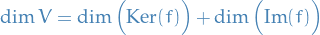
where usually we use the terminology:
- rank of is

- nullity of is

Linear Mappings and Matrices
Let be a field and let  .
.
There exists a bijection  and set of matrices with rows and
  columns:
![\begin{equation*}
\begin{split}
M: \text{Hom}_F(F^M, F^n) & \overset{\sim}{\to} \text{Mat}(n \times m; F) \\
f &\mapsto [f]
\end{split}
\end{equation*}](../../assets/latex/algebra_39c17a263e9fbcb91b2cb228766db36df4a26d2f.png)
Which attaches to each linear mapping , its representing matrix ![$M(f) := [f]$](../../assets/latex/algebra_65a75e0c78a4b206d062ea3b411f7a65611f94bf.png) , defined
, defined
![\begin{equation*}
[f] :=
\begin{pmatrix}
f(\mathbf{e}_1) & f(\mathbf{e}_2) & \dots & f(\mathbf{e}_m)
\end{pmatrix}
\end{equation*}](../../assets/latex/algebra_75ed773544a3456b1521a482b8b595409106e096.png)
i.e. the matrix-representation of is a defined by how maps the basis of the target space.
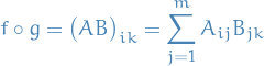
Observe that the matrix product between two matrices ![$A = [f]$](../../assets/latex/algebra_ce6900a7bef6f5274e33532d2609a40e826a1c13.png) and
and ![$B = [g]$](../../assets/latex/algebra_b68a095d4020c81ac65f4ffc446e4db613c4e15e.png) ,
,
An elementary matrix is any square matrix which differs from the identity matrix in at most one entry.
Any matrix whose only non-zero entries lie on the diagonal, and which has the first 1's along the diagonal and then 0's elsewhere, is said to be in Smith Normal Form
 there exists invertible matrices
  and
and  s.t.
s.t.  is a matrix in Smith Normal Form.
A linear mapping  is injective if and only if

Let , then

Hence, if

as claimed.
Let  be square matrices over some commutative ring
  are conjugate if

for an invertible P ∈ (n; R).
Further, conjugacy is an equivalence relation on  .
.
Trace of linear map
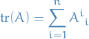
The trace of a matrix is defined
The trace of a finite product of matrices  is independent of the order of the product (given that the products are valid). In other words, trace is invariant under cyclic permutations.
To see that trace is a invariant under cyclic permutations, we observe
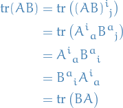
This case of two matrices can easily be generalized to case of products of multiple matrices.
Rings and modules
A ring is a set with two operatiors  that satisfy:
 is an abelian group
 is a monoid
The distributive laws hold, meaning that
 :
:
Important: in some places, e.g. earlier in your notes, they use a slightly less restrictive definition of a ring, and in that case we'd call this definition a unitary ring.
Polynomials
A field is algebraically closed if each non-constant polynomial ![$P \in F[X] \backslash F$](../../assets/latex/algebra_fb886a90b71fbee70f2c8ae6dea3e988584ec0e2.png) with coefficients in has a root in .
with coefficients in has a root in .
E.g. ![$\mathbb{C}[X]$](../../assets/latex/algebra_e100daaa67a09ac455356a0f05a0572c25ef539d.png) is algebraically closed, while
is algebraically closed, while ![$\mathbb{R}[X]$](../../assets/latex/algebra_40f5f5cfda8e63d360d33282a3238071a3d9e8e4.png) is not.
is not.
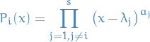
If a field is algebraically closed, then every non-zero polynomial ![$P \in F[X] \backslash \left\{ 0 \right\}$](../../assets/latex/algebra_41818dd26b791500efbe667651d828fb425a590d.png) decomposes into linear factors
decomposes into linear factors
with  ,
,  and
and  .
.
This decomposition is unique up to reordering of the factors.
![$P, Q \in R[x]$](../../assets/latex/algebra_fa38ebe1290060ad090d58f4eb95b6cc97a96984.png) with
with ![$A, B \in R[X]$](../../assets/latex/algebra_8de73281313189b1e708a2e79052789e62370129.png) such that
such that
 or
or  .
.
Ideals and Subrings
Let and  be rings. A linear map
  is a ring homomorphism if the following hold for all
  :
:
A subset  of a ring is an ideal, written
  , if the following hold:

- is closed under subtraction
 for all
  and
and  , i.e. closed under multiplication by elements of
- I.e. we stay in even when multiplied by elements from outside of
- I.e. we stay in
Ideals are sort of like normal subgroups for rings!
Let be a commutative ring and let  .
.
Then the ideal of generated by  is the set

together with the zero element in the case  .
.
If  , a finite set, we will often write


Let  be a subset of a ring . Then is a subring if and only if
- has a multiplicative identity
- is closed under subtraction:

- is closed under multiplication
It's important to note that and does not necessarily have the same identity element, even though is a subring of !
Let be a ring. An element  is a called a unit if it's invertible in or in other words has a multiplicative inverse in , i.e.

We will use the notation  for the group of units of a ring .
In a ring a non-zero element is called a zero-divisor or divisor of zero if

An integral domain is a non-zero commutative ring that has no zero-divisors, i.e.
- If
 then
then  or
or 
 and
and  then
then 
Factor Rings

Let be a ring and and ideal of  .
.
The mapping
Has the following properties:
 is surjective
If
is a ring homomorphism with  so that

then there is a unique ring homomorphism:

Where the second point states that factorizes uniquely through the canonical mapping to the factor whenever the ideal is sent to zero.
Modules
We say  is a R-module, being a ring, if
satisfying

Thus, we can view it as a "vector space" over a ring, but because it behaves wildly different from a vector space over a field, we give this space a special name: module.
Important:  denotes a module here, NOT manifold as usual.
A unitary module is in the case where we also have  , i.e. the ring is a unitary ring and contains a multiplicative identity-element.
Let be a ring and let be an R-module. A subset  of is a submodule if and only if


Let be a ring, let and be R-modules and let  be an R-homomorphism.
Then is injective if and only if

Let  . Then
  is the smallest submoduel of that contains .
The intersection of any collection of submodules of is a submodule of .
Let  and
and  be submodules of . Then

is a submodule of .
Let be a ring, and R-module and submodule of .
For ever  the coset of wrt. in is

It is a coset of in the abelian group and so is an equivalence class for the equivalence relation

The factor of by or quotient of by is the set

of all cosests of in .
Equipped with addition and s-multiplication
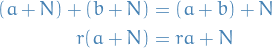
for all  and .
and .
The R-module  is the factor module of by submodule .
Let be a ring, let  and be R-modules, and a submodule of .
The mapping
 defined by

is surjective.
If
 is an R-homomorphism with

so that
 , then there is a unique homomorphism
  such that
  .
.
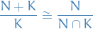
Let be a ring and let and be R-module. Then every R-homomorphism induces an R-isomorphism
Let  be submodules of a R-module .
Then is a submodule of  and
and  is a submodule of .
Also,
Let be submodules of an R-module , where  .
.
Then  is a submodule of
  .
.
Also,

Determinants and Eigenvalue Reduction
Definitions
An inversion of a permutation  is a pair
  such that
  and
and  .
.
The number of inversions of the permutation  is called the length of and writtein
  .
.
The sign of a permutation is defined to be the parity of the number of inversions of :
where  is the length of the permutation.
For  , the set of even permutations in
  forms a subgroup of because it is the kernel of the group homomorphism
  .
.
This group is the alternating group and is denoted  .
.
(X̃ / ker(p))
Let be a ring.
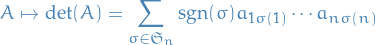
The determinant is a mapping  given by
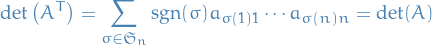
Let be a commutative ring, then
Let  for some ring , and let
  be the
  defined by removing the i-th row and j-th column of .
Then the cofactor matrix  of is defined (component-wise)

The adjugate matrix of is defined

where is the cofactor matrix.
The reason for this definition is so that we have the following identity

To see this, recall the "standard" approach to computing the determinant of a matrix , where we do so by choosing some row  and some column
  , cut out the rest of the matrix, and write the determinant as a expansion in these coefficients. The cofactor matrix has exactly the determinant of that matrix as a entries, hence the above expression is simply going to give us the same expression as the "expansion-method" for computing the determinant.
Let  be an
be an  matrix with entries from a commutative ring .
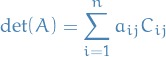
For a fixed the i-th row expansion of the determinant is
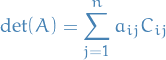
and for a fixed the j-th column expansion of the determinant is
where  is the cofactor of

where  is the matrix obtained from deleting the i-th row and j-th column.
Cayley-Hamilton Theorem
Let be a square matrix with entries in a commutative ring .
Then evaluating its characteristic polynomial ![$\chi_A(x) \in R[x]$](../../assets/latex/algebra_92f22474b9af5baaae581bd27764aefbe2b62aff.png) at the matrix gives zero.
at the matrix gives zero.
Let
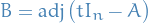
where  denotes the adjugate matrix of
  and
and  .
.
Observe then that

by the propoerty of the adjugate matrix.
Since  is a matrix whose entries are a polynomial, we can write as
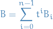
for some matrices 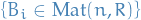 .
.
Therefore,
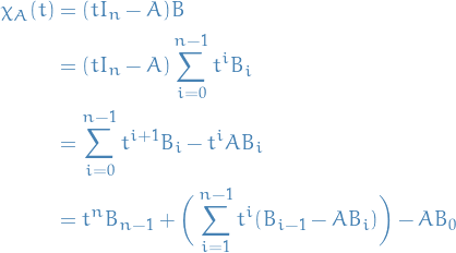
Now, letting

we obtain the following relations
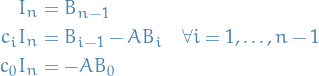
Multiplying the above relations by  for each we get the following
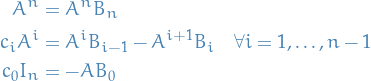
Substituting back into the above series, we have

we observe that the LHS vanishes, since we can group terms which cancel! Hence

Eigenvalues and Eigenvectors
Theorems
Each endomorphism of non-zero finite dimensional vector space over an algebraically closed field has an eigenvalue.
Inner Product Spaces
Definitions
Inner product
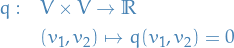
An inner product is a (anti-)bilinear map  which is
- Symmetric
- Non-degenerate
- Positive-definite
Forms
Let  . We say is a bilinear form if
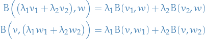
for  ,
,  and
and  .
.
A symmetric bilinear form on  is a bilinear map
  such that
  .
.
Given two 1-forms  at
at  define a symmtric bilinear form
  on
on  by
by
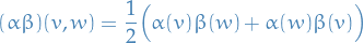
where  .
.
Note that  and we denote
  .
.
REDEFINE WITHOUT THE ADDED TANGENT-SPACE STRUCTURE, BUT ONLY USING VECTOR SPACE STRUCTURE.
A symmetric tensor on  is a map which assigns to each a symmetric bilinear form on ; it can be written as
where  are smooth functions on .
Remember, we're using Einstein notation.
Skew-linear and sesquilinear form
We say the mapping between complex vector spaces is skew-linear if
Let be a vector space over  equipped with the inner product

Since this mapping is skew-linear in the second argument, i.e.

we say this is a sesquilinear form.
Hermitian
 is symmetric, i.e.

 is a Hermitian.
Theorems
Let  be a vectors in an inner product space. Then

with equailty if and only if  and
and  are linearly dependent.
Adjoints and Self-adjoints
Let be an inner product space. then two endomorphism  are called adjoint to if the following holds:

Let  and
and  be the adjoint of . We say is self-adjoint if and only if

Let be a finite-dimensional inner product space and let be a self-adjoint linear mapping.
Then has an orthonormal basis consisting of eigenvectors of .
We'll prove this using induction on  . Let
. Let  denote the an inner product space with
  with the self-adjoint linear mapping .
Base case:  .
Let
.
Let  denote an eigenvector of , i.e.

where is the underlying field of the vector space . Then clearly  spans .
General case: Assume the hypothesis holds for  , then

where

Further, let  and
and  with
with  be an eigenvector of . Then

since is self-adjoint. This implies that

Therefore, restricting to  we have the mapping
Where  is also self-adjoint, since is self-adjoint on the entirety of
  . Thus, by assumption, we know that there exists a basis of consisting of eigenvectors of , which are therefore orthogonal to the eigenvectors of in . Hence, existence of basis of eigenvectors for implies existence of basis of eigenvectors of .
Thus, by the induction hypothesis, if is a self-adjoint operator on the inner product space with  , , then there exists a basis of eigenvectors of for , as claimed.
Jordan Normal Form
Notation
 is an endomorphism of the finite dimensional F-vector space .
Characteristic equation of
 :
:
![\begin{equation*}
\chi_{\phi}(x) = \big( \lambda_1 - x \big)^{a_1} \big( \lambda_2 - x \big)^{a_2} \cdots \big( \lambda_s - x \big)^{a_s} \in F[x]
\end{equation*}](../../assets/latex/algebra_a6e0c2cd5b6fc3f9ed9dcf6ca50f1e6ef5a8da83.png)
Polynomials
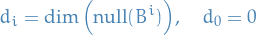
Generalized eigenspace of
wrt. eigenvalue 

 denotes the dimension of
Basis

Restriction of

 defined

is well-defined and injective.

Definitions
An endomorphism  of an F-vector space is called nilpotent if and only if
  such that

Motivation
- be a finite dimensional vector space
- an endomorphism
- a choice of ordered basis for determines a matrix
![$~_{\mathcal{B}} [f]_{\mathcal{B}}$](../../assets/latex/algebra_a0841be11b162a5f21684e66cd4bbb4945c870dc.png) representing wrt. basis
representing wrt. basis
- a choice of ordered basis
- Another choice of basis leads to a different representation; would like to find the simplest possible matrix that is conjugate to a given matrix
Theorem
Given an integer  , we define the
  matrix
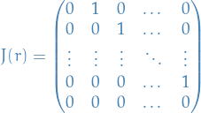
or equivalently,
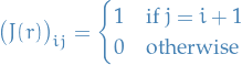
which we call the nilpotent Jordan block of size .
Given an integer and a scalar  define an matrix
  as
as
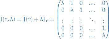
which we is called the Jordan block of size and eigenvalue  .
.
Let be an algebraically closed field, and be a finite dimensional vector space and be an endomorphism of with characteristic polynomial
![\begin{equation*}
\chi_{\phi}(x) = \big( \lambda_i - x \big)^{a_1} \big( \lambda_2 - x \big)^{a_2} \cdots \big( \lambda_s - x \big)^{a_s} \in F[x]
\end{equation*}](../../assets/latex/algebra_e1a53a69bbd5627923568c535b83662d5601988c.png)
where  and
and  , for distinct
  .
.
Then there exists an ordered basis of s.t.
![\begin{equation*}
~_{\mathcal{B}}[\phi]_{\mathcal{B}} = \text{diag} \Big( J(r_{11}, \lambda_1), \dots, J(r_{1 m_1}, \lambda_1), J(r_{21}, \lambda_2), \dots, J(r_{s m_s}, \lambda_s) \Big)
\end{equation*}](../../assets/latex/algebra_05ed2912f98e30105137f8a206da16019fc0403a.png)
with  such that

with  .
.
That is, in the basis is block diagonal with Jordan blocks on the diagonal!
Proof of Jordan Normal Form
- Outline
We will prove the Jordan Normal form in three main steps:
Decompose the vector space
into a direct sum

according to the factorization of the characteristic polynomial as a product of linear factors:
![\begin{equation*}
\chi_{\phi}(x) = \big( \lambda_1 - x \big)^{a_1} \big( \lambda_2 - x \big)^{a_2} \cdots \big( \lambda_s - x \big)^{a_s} \in F[x]
\end{equation*}](../../assets/latex/algebra_b54120af1b855bb5c6cd87af6b184bc83bfbdf6c.png)
for distinct scalars
, where for each :
- Focus attention on each of the
 to obtain the nilpotent Jordan blocks.
 - Combine Step 2 and 3
- Step 1: Decompose
Rewriting
 as
as
![\begin{equation*}
\chi_{\phi}(x) = (-1)^n \prod_{j = 1}^s \big( x - \lambda_j \big)^{a_j} \in F[x]
\end{equation*}](../../assets/latex/algebra_c4013d57b73134bd93174af5478306011fe6127a.png)
where
 are the eigenvalues of .
For
define
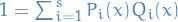
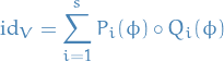
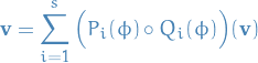
There exists polynomials
![$Q_i(x) \in F[x]$](../../assets/latex/algebra_32c1fc31e99cf3fb193b232e2facf657e1b59eab.png) such that
such that
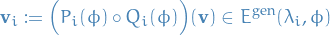
For each
, let

be a basis of
, where is the algebraic multiplicity of with eigenvalue .
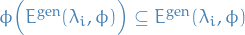
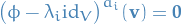
- Each is stable under , i.e.
For each
,  such that

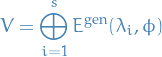
In other words, there is a direct sum decomposition

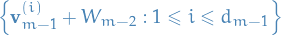
Then

is a basis of
, so in particular 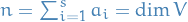 .
The matrix of the endomorphism wrt. to basis is given by the block diagonal matrix
.
The matrix of the endomorphism wrt. to basis is given by the block diagonal matrix
![\begin{equation*}
~_{\mathcal{B}}[\phi]_{\mathcal{B}} =
\left(
\begin{array}{c|c|c|c}
B_1 & 0 & 0 & 0 \\
\hline
0 & B_2 & 0 & 0 \\
\hline
0 & 0 & \ddots & 0 \\
\hline
0 & 0 & 0 & B_s
\end{array}
\right)
\in \text{Mat}(n; F)
\end{equation*}](../../assets/latex/algebra_c02066ebcd6aed4e5ad9ad676c504f6743b1c78d.png)
with
![$B_i = ~_{\mathcal{B}}[\phi_i]_{\mathcal{B}} \in \text{Mat}(a_i; F)$](../../assets/latex/algebra_4e8e2a19c239252a2bec5dc9c2e4dd64341dc9da.png) .
.
Let
 is that
Then

Hence
 , i.e. is stable under .
By Lemma 6.3.1 we have
 and so evaluating this at , we get
Therefore,
 , we have
Observe that

where we've used Cailey-Hamilton Theorem for the second equality. Let
then

hence all
can be written as a sum of  , or equivalently,
as claimed.
Since
 is a basis of for each , and since

we have

form a basis of
.
Consider the ordered basis  , then the
  can be expressed as a linear combination of the vectors
  with
with  . Therefore the matrix is block diagonal with i-th block having size
  .
.
From this, one can prove that any matrix
can be written as a Jordan decomposition:
Let
 , then there exists a diagonalisable (NOT diagonal) matrix and nilpotent matrix such that

In fact, this decomposition is unique and is called the Jordan decomposition.
- Each
- Step 2: Nilpotent endomorphisms
Let
be a finite dimensional vector space and  such that

for some
 , i.e.
  is nilpotent. Further, let be minimal, i.e.
  but
but  .
.
For
 define

If
 then
then

i.e.
 , hence

Moreover, since
 and
and  , we have
  and
and  . Therefore we get the chain of subspaces

We can now develop an algorithm for constructing a basis!
- Constructing a basis
- Choose arbitrary basis
 for
for 
- Choose basis of
 of
of  by mapping using
  and choosing vectors linearly independent of
  .
. - Repeat!
Or more accurately:
Choose arbitrary basis for
:

Since
 is injective, by the fact that the image of a set of linear independent vectors is a linearly independent set if the map is injective, then

is linearly independent.
Choose vectors
such that
is a basis of
 .
.
- Repeat!
Now, the interesting part is this:
Let
be a finite dimensional vector space and such that
for some
, i.e. is nilpotent.
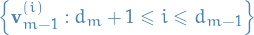
Let
be the ordered basis of constructed as above
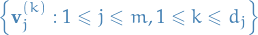
Then
![\begin{equation*}
~_{\mathcal{B}}[\psi]_{\mathcal{B}} = \diag \Big( \underbrace{J(m), \dots, J(m)}_{d_m \text{ times}}, \underbrace{J(m - 1), \dots, J(m - 1)}_{d_{m - 1} - d_m \text{ times}}, \dots, \underbrace{J(1), \dots, J(1)}_{d_1 - d_2 \text{ times}} \Big)
\end{equation*}](../../assets/latex/algebra_4edc751c9e7702a08963fb883685d09e5fca763a.png)
where
denotes the nilpotent Jordan block of size .
It follows from the explicit construction of the basis
that
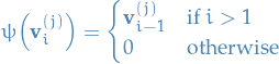
Since
![$~_{\mathcal{B}}[\psi]_{\mathcal{B}}$](../../assets/latex/algebra_709e9b66cf9d42445a73e4468667cefc6dbd2bda.png) is defined by how it maps the basis vectors in , and in the basis
is defined by how it maps the basis vectors in , and in the basis  becomes a vector of all zeros except the entry corresponding to the j-th basis-vector chosen for
  , where it is a 1.
Hence
is a nilpotent Jordan block as claimed.
Concluding step 2; for all nilpotent endomorphisms there exists a basis such that the representing matrix can be written as a block diagonal matrix with nilpotent Jordan blocks along the diagonal.
- Choose arbitrary basis
- Constructing a basis
- Step 3: Bringing it together
Again considering the endomorphisms
 restricted to , we can apply Proposition 6.3.9 to see that this endomorphism can be written as a block diagon matrix of the form stated for a suitable choice of basis.
The endomorphism
 restricted to is of course
  , thus the matrix wrt. the chosen basis is just
  . Therefore the matrix for
  (when restricted to ) is just plus
  , i.e.
  .
.
Thus, each
 appearing in this theorem is exactly of the form we stated in Jordan Normal form.

Algorithm
Calculate the eigenvalues,
 of
of

For each
 and
and  , let
, let

Compute
 and
and

Let
Set

i.e. the difference in dimension between each of the nullspaces.
- Let be the largest integer such that
 .
. - If
 does not exist, stop.
Otherwise, goto step 3.
does not exist, stop.
Otherwise, goto step 3. - Let
 and
and  .
. - Let

- Change
 to
to  for
for  .
.
- Let
- Let the full basis be the union of all the , i.e.
 .
.
Tensor spaces
The tensor product  between two vector spaces is a vector space with the properties:
- if
 and
and  , there is a "product"
This product
 is bilinear:
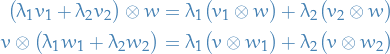
for
, and .
 be a
be a 
I find the following instructive to consider.
In the case of a Cartesian product, the vector spaces are still "independent" in the sense that any element can be expressed in the basis

which means

Now, in the case of a tensor product, we in some sense "intertwine" the spaces, making it so that we cannot express elements as "one part from and one part from ". And so we need the basis

Therefore

By universal property of tensor products we can instead define the tensor product between two vector spaces as the dual vector space of bilinear forms on  .
.
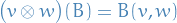
If , , then is defined as the map

for every bilinear form .
That is,

and

by
Observe that this satisfies the universal property of tensor product since if we are given some  , for every
  , i.e.
  , we have
  , i.e.
  is a bilinear form on . Furthermore, this dual of bilinear forms on is then
  (since we are working with finite-dimensional vector spaces).

From universal property of tensor product, for any , there exists a unique  such that

Letting the map

be defined by

where  is defined by
  . By the uniqueness of
  , and linearity of the maps under consideration, this defines an isomorphism between the spaces.
Suppose
 is a basis for
  is a basis for
Then a bilinear form is fully defined by  (upper-indices since these are the coefficients of the co-vectors). Therefore,

Since we are in finite dimensional vector spaces, the dual space then has dimension

as well.
Furthermore,  form a basis for . Therefore we can write the elements in as
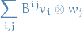

First observe that if  , then is fully defined by how it maps the basis elements
  , and
, and

Then observe that if  , then
Hence, we have a natural homomorphism which simply takes , with coefficients  to the corresponding element
  with the same coefficients! That is, the isomorphism is given by

Tensor algebra
Now we'll consider letting  . We define tensor powers as

with  ,
,  , etc.
We can think of
, etc.
We can think of  as the dual vector space of k-multilinear forms on .
Combining all tensor powers using the direct sum we have define the tensor algebra
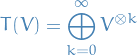
whose elements are finite sums
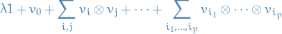
of tensor products of vectors  .
.
The "multiplication" in  is defined by extending linearly the basic product

The resulting algebra is associative, but not commutative.
Two viewpoints
There are mainly due two useful ways of looking at tensors:
Using Lemma lemma:homomorphisms-isomorphic-to-1-1-tensor-product, we may view
 tensors as linear maps
  . In other words,

- Furthermore, we can view
 as the dual of
 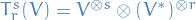 , i.e. consider a
  tensor as a "multilinear machine" which takes in
  vectors and co-vectors, and spits out a real number!
- Furthermore, we can view
- By explicitly considering bases
 of and
  of
of  , the tensors are fully defined by how they map each combination of the basis elements. Therefore we can view tensors as multi-dimensional arrays!
Tensors (mainly as multidimensional arrays)
Let be a vector space  where is some field,
  is addition in the vector space and
  is scalar-multiplication.
Then a tensor is simply a linear map from some q-th Cartesian product of the dual space and some p-th Cartesian product of the vector space to the reals  . In short:

where  denotes the (p, q) tensor-space on the vector space , i.e. linear maps from Cartesian products of the vector space and it's dual space to a real number.
Tensors are geometric objects which describe linear relations between geometric vectors, scalars, and other tensors.
A tensor of type  is an assignment of a multidimensional array
![\begin{equation*}
T_{j_1, \dots, j_q}^{i_1, \dots, i_p} [ \mathbf{f} ]
\end{equation*}](../../assets/latex/algebra_4636b2bb9b5133c787efc5f0063b4b8d040bc734.png)
to each basis  of an n-dimensional vector space such that, if we apply the change of basis
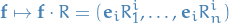
Then the multi-dimensional array obeys the transformation law
![\begin{equation*}
T_{j'_1 \dots, j'_p}^{i'_1, \dots, i'_q} [\mathbf{f} \cdot R] = \big( R^{-1} \big)_{i_1}^{i'_1} \dots \big( R^{-1} \big)_{i_p}^{i'_p} \
T_{j_1, \dots, j_q}^{i_1, \dots, i_p} [ \mathbf{f} ] \
R_{j'_1}^{j_1} \dots R_{j'_q}^{j_q}
\end{equation*}](../../assets/latex/algebra_db97bd8ea12841f1c2aac31a4c97d6146d2cfe89.png)
We say the order of a tensor is if we require an n-dimensional array to describe the relation the tensor defines between the vector spaces.
Tensors are classified according to the number of contra-variant and co-variant indices, using the notation , where
- is # of contra-variant indices
 is # of co-variant indices
Examples:
- Scalar :

- Vector :

- Matrix :

- 1-form:

- Symmetric bilinear form:

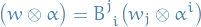
The tensor product takes two tensors, and , and produces a new tensor,  , whose order is the sum of the orders of the original tensors.
When described as multilinear maps, the tensor product simply multiplies the two tensors, i.e.

which again produces a map that is linear in its arguments.
On the components, this corresponds to multply the components of the two input tensors pairwise, i.e.

where
- is of type

- is of type

Then the tensor product is of type  .
.
Let  be a basis of the vector space with , and
  be the basis of .
Then  is a basis for the vector space of
  over , and so

Given  , we define


Components:

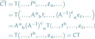
A contraction is basis independent:
![\begin{equation*}
\begin{split}
\tensor{T}{_{(a, b)}} &= \frac{1}{2} \big( \tensor{T}{_{ab}} + T_{ba} \big) \implies T_{(a, b)} = T_{(b, a)} \\
\tensor{T}{_{[a, b]}} &= \frac{1}{2} \big( \tensor{T}{_{ab}} - \tensor{T}{_{ba}} \big) \implies T_{[a, b]} = - T_{[b, a]}
\end{split}
\end{equation*}](../../assets/latex/algebra_b9131aa9bf3922b3d3c0d9cbcef308cfd5df2086.png)
Generalized to by summing over combinations of the indices, alternating sign if wanting anti-symmetric. See the general definition of a wedge product for more for example.
Clifford algebra
First we need the following definition:
Given a commutative ring and modules M$ and , an quadratic function  s.t.
s.t.
(cube relation): For any
 we have

(homegenous of degree 2): For any
 and any , we have
A quadratic R-module is an module equipped with a quadratic form: an R-quadratic function on with values in .
The Clifford algebra  of a quadratic R-module
  can be defined as the quotient of the tensor algebra
  by the ideal generated by the relations
  for all ; that is

where  is the ideal generated by .
In the case we're working with a vector space (instead of a module), we have

Since the tensor algebra is naturally  graded, the Clifford algebra
  is naturally
  graded.
Examples
Exterior / Grassman algebra
Consider a Clifford algebra
generated by the quadratic form
i.e. identically zero.
- This apparently gives you the Exterior algebra over
- A bit confused as to why