Geometry
Table of Contents
- Notation
- Stuff
- Definitions
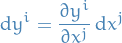
- Words
- Regular curves
- Level set
- Arc-length
- Curvature
- Torsion
- Isometry
- Tangent spaces
- Tangent bundle
- Cotangent bundle
- Dual space
- 1-forms
- k-form
- Wedge product
- Multi-index
- Differential k-form
- Exterior derivative
- Integration in Rn
- Topological space
- Atlases & coordinate charts
- Manifolds
- Diffeomorphism
- Isometric
- Algebra
- Equations / Theorems
- Change of basis
- Determinants
- Tangent space and manifolds
- Tensor Fields and Modules
- Grassman algebra and deRham cohomology
- Lie Theory
- Notation
- Stuff
- Examples of Lie groups
- Classification of Lie Algebras
- Representation Theory of Lie groups and Lie algebras
- Reconstruction of Lie group from it's Lie algebra
- Lie group action, on a manifold
- Structure theory of Lie algebras
- Parallel Transport
- Curvature and torsion (on principle G-bundles)
- TODO Covariant derivatives
- Spinors on curves spaces
- Relating to Quantum Mechanics
- Complex dynamics
- Partitions of Unity
- Integration
- Cartan calculus
- Temp
- Q & A
- Bibliography
Notation
 denotes the space of all functions which have continuous derivatives to the k-th order
- smooth means
 , i.e. infitively differentiable, more specificely,
  means all infitively differentiable functions with domain
- Maps
 are assumed to be smooth unless stated otherwise, i.e. partial derivatives of every order exist and are continuous on
 - Euclidean space
 as the set
  together with its natural vector space operations and the standard inner product
 - sub-scripts (e.g. basis vectors
 for
for  and coeffs.
  for
for  ) are co-variant
 - super-scripts (e.g. basis vectors of
 for and coeffs
  for ) are contra-variant
  where
where  are manifolds, uses the
  to refer to a linear map from
  to
to 
Stuff
Curves
Examples
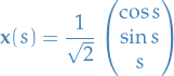
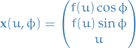
Helix
The helix in  is defined by
Constructing a sphere in Euclidean space
I suggest having a look at this page in the notes
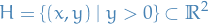
Surface of a sphere in the Euclidean space is defiend as:
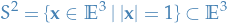
As it turns out,  is not a vector space. How do you define vectors on this spherical surface ?
Defining vectors on spherical surface
At each point on , construct a whole plan which is tangent to the sphere, called the tangent plane.
This plane  is the two dimensional vector space of lines tangent to the sphere at the given point, called tangent vectors.
Each point on the sphere defines a different tangent plane. This leads to the notion of a vector field which is: a rule for smoothly assigning a tangent vector to each point on .
The above description of a vector space on is valid everywhere, and so we refer to it as a global description.
Usually, we don't have this luxury. Then we we parametrise a number of "patches" of the surface using coordinates, in such a way that the patches cover the whole surface. We refer to this as a local description.
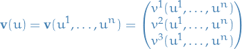
Motivation
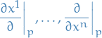
The tangent-space  at some point
  on the 2-sphere is a function of the point .
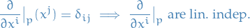
The issue with the 2-sphere is that we cannot obtain a (smooth) basis for the surface. We therefore want to think about the operations which do not depend on having a basis. gives a way of doing this, since each of the derivatives are linear inpendent.
Ricci calculus and Einstein summation
This is reason why we're using superscript to index our coordinates,  .
.
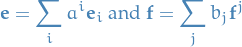
Suppose that I have a vector space and dual space . A choice of basis  for induces a dual basis
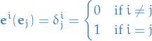
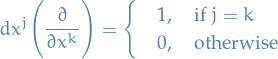
  on the dual vector space , determined by the rule

where  is the Kronecker delta.
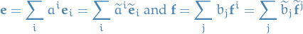
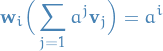
Any element  of or
of or  of can be written as lin. comb. of these basis vectors:
and we have 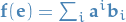 .
.
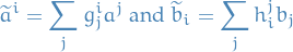
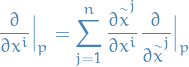
If we do a change of basis of , which induces a change of basis for , then the coefficients of a vector in transform in the same way as the basis of vectors and vice versa, the coefficients of a vector transform in the same way as the basis vectors of .
Suppose a new basis for is given by  , with
where the  are the coefficients of the invertible change-of-basis matrix, and
  are the coefficients of its inverse (i.e.
 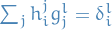 ). If we denote the new induced dual basis for by
  , we have
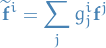
Moreover, for any elements of of and of which we can write as
we have
See how the order of the indices are different?
The entities and are co-variant .
The entities and are contra-variant .
One-forms are sometimes referred to as co-vectors , because their coefficients transform in a co-variant way.
The notation then goes:
- sub-scripts (e.g. basis vectors for and coeffs. for ) are co-variant
- super-scripts (e.g. basis vectors of for and coeffs for ) are contra-variant
Very important: "super-script indicies in the denominator" are understood to be lower indices, i.e. co-variant in denominator equals contravariant.
Now, consider this notation for our definition of tangent space and dual space:
If you choose coordinates  on an open set
  containing a point , then you get a basis for the tangent space at
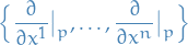
which have super-script in denominator, indicating a co-variant entity (see note).
Similarily we get a basis for the cotangent space  at
at
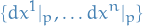
which have super-script indices, indicating a contra-variant entity.
Why did we decide the first case is the co-variant (co- and contra- are of course relative)?
Because in differential geometry the co-variant entities transform like the coordinates do, and we choose the coordinates to be our "relative thingy".
Differential forms
Differential forms are an approach to multivariable calculus which is independent of coordinates.
Surfaces
Notation
 is the domain in the plane whose Cartesian coordinates will be denoted
  unless otherwise stated
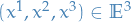 , unless otherwise stated
 denotes the image of the smooth, injective map
Regular surfaces
A local surface in is smooth, injective map with a continuous inverse of  . Sometimes we denote the image by
  .
.
The assumptation that  is injective means that points in the image are uniquely labelled by points in .
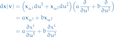
Given a local surface we define

For every point  , these are vectors in
  , which we will identify with itself.
We say that a local surface is regular at if
, which we will identify with itself.
We say that a local surface is regular at if  and
and  are linearly independent.
A local surface is regular if it is regular at for all .
are linearly independent.
A local surface is regular if it is regular at for all .
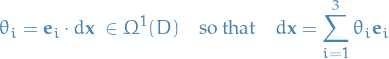
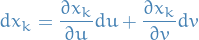
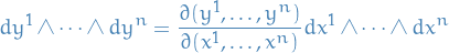
This gives rise to the differential form  :
:

Here is a quick example of evaluating the differential form induced by the definition of a regular local surface:
 is a regular surface if for each
  there exists a regular local surface such that
  and
and 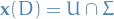 for some open set
  .
.
In other words, if for each point on the surface we can construct a regular local surface, then the entire surface is said to be regular.
A map defines a local surface which is part of some surface  , is sometimes called a coordinate chart on .
Thus, if the surface is a regular surface (not just locally regular) we can "define" from a set of all these coordinate charts .
At a regular point on a local surface, the plane spanned by and  is the tangent plane to the surface at
  , which we denote by
  . At a regular point, the unit normal to the surface is
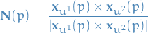
Clearly,  is orthogonal to the tangent plane .
Given a local surface the map  is a smooth function whose image lies in a unit sphere
  . The map
  is called the local Gauss map.
Standard Surfaces
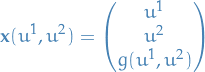
Let  be a smooth function. The graph of
  is the local surface defined by
An implicitly defined surface is zero set of a smooth function  , i.e.

Note that  is a mapping from , and we're saying that the inverse of this function defines a surface, where it's also important to note the smooth requirement, as this implies that is differentiable.
An implicitly defined surface  , such that
  everywhere
on , is a regular surface.
everywhere
on , is a regular surface.
This is due to the fact that if there is a point such that  , then that implies that
  and
and  are linearly dependent, hence not a regular surface.
A surface of revolution with profile curve  is a local surface of the form
A surface of revolution can be constructed by rotation a curve  around the
  axis in
  . It thus has cylindrical symmetry.
A ruled surface is a surface of the form
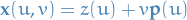
Notice that curves of constant  are straight lines in through
  in the direction
  .
.
Examples of surfaces
Quadratic surfaces
Quadratic surfaces are the graphs of any equation that can be put into the general form:
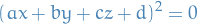
The general equation for a cone
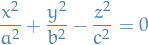
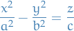
The general equation for a hyperboloid of one sheet
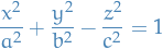

The general equation for a hyperboloid of two sheets
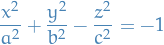

The general equation for an ellipsoid
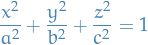
with  being a sphere.
General equation for an elliptic paraboloid
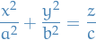

General equation for an hyperbolic paraboloid

Fundamental forms
Symmetric tensors
Notation

 are coordinates
Definitions
A (Riemannian) metric on is a symmetric tensor  which is positive definite at each point;
  , with equality if and only if
  .
.
Equivalently, it is a choice for each of an inner product on
First fundamental form
Notation
- and
 are our coordinates
Stuff
This bijectivity can be used to give a coordinate free definition of regularity of a local surface.
Given a regular local surface , the first fundamental form is defined by

where we have introduced the notation  .
.

 are functions on
The first fundamental form is a metric on .
 be a vector field on
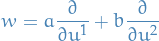

 implies
  , so the map is one-to-one.
Second Fundamental form
Notation
- and are our coordinates
- is the normal of the surface (if my understanding is correct)
Stuff
Given a local surface , the second fundamental form is defined by

with the dot product interpreted as usual.
The valued 1-form  is linear map which may have a non-trivial kernel. It is convenient to use the isomorphism
  to rewrite the map as a symmetric bilinear form.
Since is unit normalised it follows that  (by differentiating
  by
by  and
and  respectively).
Hence,  and
and  must belong to the tangent plane
  . In other words,
  .
.
The second fundamental form is given by

where  are continuous functions on given by

Which can also be written as

Q & A
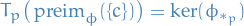
- DONE What do we mean by a 1-form having a "non-trivial kernel"?
In Group-theory we have the following definition of a kernel :

where
 is a homomorphism.
When we say the mapping
 has a non-trivial kernel, we mean that there are more elements in
  than just the identity element which is being mapped to the identity-element in
  , i.e.

Hence, in the case of the some 1-form
, we have mean

i.e. non-trivial kernel refers to the 1-form mapping more than just the zero-vector to the zero-vector in the target vector-space.
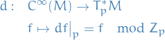
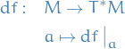
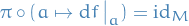
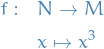
- DONE What do we mean when we write dx from TpD to Tx(p) S?
What do we mean when we write the following:

where:
 is some surface in
 - is the domain of our "coordinates"
- is a smooth map
Curvature
Notation
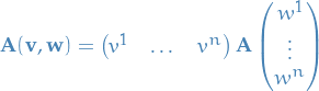
 are symmetric bilinear forms on a real vector space , which we can represent in matrix form as:
 is a basis of
  represents the principal curvatures
Bilinear algebra
The eigenvalues of  wrt.
wrt.  are roots of the polynomial

where are represented by symmetric  matrices.
If is positive definite (i.e.  defines an inner product) there exists a basis
  of such that:
- is orthonormal wrt.
- each
 is an eigenvector of wrt. with a real eigenvalue
Gauss and mean curvatures
 have 2 symmetric bilinear forms on
  ,
,  and
and  look for eigenvalues & eigenvectors of and .
The eigenvalues of wrt. are the principal curvatures of the surface. The corresponding eigenvectors are the principal directions of the surface. Hence the principal curvatures are the roots of the polynomial  .
.
The principal curvatures may vary with position and so are (smooth) functions on .
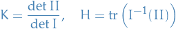
The product of the principal curvatures is the Gauss curvature :

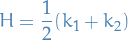
Average of the principal curvatures is the Mean curvature :
If  we have that all directions are principal.
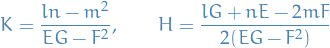
where all variables are as given by the first and second fundamental forms.
We get the elegant basis independent expressions
Thus, the Gauss curvature is positive if and only if is positive definite.
Meaning of curvature
Notation
- is the domain of the plane with coordinates

 be a regular local surface
![$c:[a, b] \to D$](../../assets/latex/geometry_72874374fa11c82f125fb710232b4461655d7653.png) given by the map
given by the map 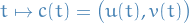 is a regular curve in
 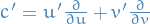 is the tangent-vector of the curve
Curves on surfaces
The composition
![\begin{equation*}
\mathbf{x} \circ c : [a, b] \to \mathbb{E}^3, \quad t \mapsto \mathbf{x}\big(c(t)\big)
\end{equation*}](../../assets/latex/geometry_ba543ff5b7e3840f5ad88345dbb3eb313fe92a9b.png)
describes a curve in lying on the surface.
and
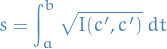
The arclength of the curve ![$\mathbf{x}\big( c(t) \big), \quad t \in [a, b]$](../../assets/latex/geometry_707cefbe575c0da587357b01136798bd13d9fd39.png) , lying on the surface is
, lying on the surface is
Invariance under Euclidean motions
Let and  be two surfaces related by a Euclidean motion, so

where  is a orthogonal matrix with
  and
and  .
.
Then,
and hence, in particular,

The first fundamental form and second fundamental form determine the surface (up to Euclidean motions).
Taylor series
Let  be a point on a regular local surface. By Euclidean motion, choose
  to be at the origin, and the unit normal at that point to be along the positive axis so
  is the
  plane.
Near we can parametrise the surface as a graph:

where at the origin
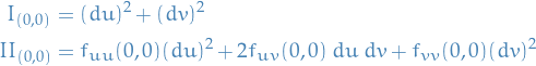
Using the above parametrization, and observing that  and
and  span
span  , which is the plane orthogonal to
  , we see that
  and
and  .
.
Further, supposing the  axes correspond to the principal directions, then the Taylor series of the surface near the origin is
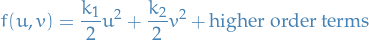
where are the principal curvatures at .
Umbilical points
Let  be a regular local surface.
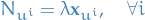
We then say a point is a umbilical if and only if

or equivalently,

i.e. all directions are pricipal directions.
An umbilical point is part of a sphere.
We can see the "being a part of a sphere" from the fact that a point on a sphere can be written as
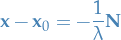
where  corresponds to pointing inwards, while
  is pointing outwards. In this case, we have

hence,

Conversely, if  then
then

Which tells us that
Thus,

where  is just some constant. Then,

A regular local surface has  if and only if it is (a piece of) a plane.
The statement that  or
or  is equivalent of saying that is part of a plane, since the tangents of the map are perpendicular to the normal.
Every point is umbilical if and only if the surface is a plane or a sphere.
If  for some smooth function
  , then

(here we have  as a function, thus the exterior derivative of gives us a 1-form).
And since

and hence by regularity of the surface  . Thus is a constant function on which implies
  .
.
This is because we've already stated that if  is part of a plane (thm:second-fundamental-form-zero-everywhere-on-surface) and if
  and constant we have to be part of a sphere (thm:all-points-umbilical-surface-is-sphere-or-plane).
Problems
Lemma 9.1 (in the notes)

![\begin{equation*}
\begin{split}
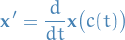
\frac{d}{dt} \mathbf{x} \big( c(t) \big) &= \frac{\partial x^i}{\partial t} \frac{\partial}{\partial x^i} \\
&= \bigg( \frac{\partial x^i}{\partial u} \frac{\partial u}{\partial t} \bigg) \frac{\partial}{\partial x^i} + \bigg( \frac{\partial x^i}{\partial v} \frac{\partial v}{\partial t} \bigg) \frac{\partial}{\partial x^i} \qquad \text{(by chain rule)} \\
&= \mathbf{x}_u u'(t) + \mathbf{x}_v v'(t) \qquad \qquad \qquad \qquad \qquad \bigg( \frac{du}{dt} = u'(t) \bigg) \\
&= \mathbf{x}_u u'(t) \bigg( du \frac{\partial}{\partial u} \bigg) + \mathbf{x}_v v'(t) \bigg( dv \frac{\partial}{\partial v} \bigg), \qquad \bigg( dv \frac{\partial}{\partial v} = 1 \bigg) \\
&= d \mathbf{x} \Bigg[ u'(t) \frac{\partial}{\partial u} + v'(t) \frac{\partial}{\partial v} \Bigg] \\
&= d \mathbf{x} \big( c'(t) \big)
\end{split}
\end{equation*}](../../assets/latex/geometry_2c48634547b2e9f574736880e760809f7b45f7bd.png)
![\begin{align*}
\frac{d}{dt} \mathbf{x} \big( c(t) \big) &= \frac{\partial x^i}{\partial t} \frac{\partial}{\partial x^i} \\
&= \bigg( \frac{\partial x^i}{\partial u} \frac{\partial u}{\partial t} \bigg) \frac{\partial}{\partial x^i} + \bigg( \frac{\partial x^i}{\partial v} \frac{\partial v}{\partial t} \bigg) \frac{\partial}{\partial x^i}, & \text{(by chain rule)} \\
&= \mathbf{x}_u u'(t) + \mathbf{x}_v v'(t), & \bigg( \frac{du}{dt} = u'(t) \bigg) \\
&= \mathbf{x}_u u'(t) \bigg( du \frac{\partial}{\partial u} \bigg) + \mathbf{x}_v v'(t) \bigg( dv \frac{\partial}{\partial v} \bigg), & \bigg( dv \frac{\partial}{\partial v} = 1 \bigg) \\
&= d \mathbf{x} \Bigg[ u'(t) \frac{\partial}{\partial u} + v'(t) \frac{\partial}{\partial v} \Bigg] \\
&= d \mathbf{x} \big( c'(t) \big)
\end{align*}](../../assets/latex/geometry_5c1c6bd3ef571c61e7048498f8aab76bd3170e1a.png)
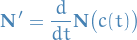
Moving frames in Euclidean space
Notation
 is a smooth map
 denotes the coordinates on
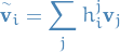
- moving frame denotes a collection of maps
 for
for  such that these form a oriented orthonormal basis of
 - oriented means that
 , which, because the frame is oriented, we have
  , i.e. it's a rotation matrix
Stuff
A moving frame for on is a collection of maps for such that for all  the
the  form an oriented orthonormal basis of .
Oriented means that .
This definition uses the notation of orientedness in three dimensions. For general  there is a different definition of a oriented frame.
If  , given by
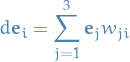
we write  for its entry by entry exterior derivative:
Thus, takes vector fields in and spits out vectors in .
Connection forms and the structure equations
Since  is an orthonormal basis for , any vector
  can be expanded as
  in the moving frame, and the same applies to a vector-valued 1-form, e.g. .
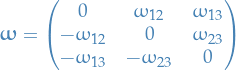
Therefore we define 1-forms  by
by
The 1-forms 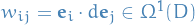 are called the connection 1-forms and by definition satisfy
Each  are in this case a 1-form.
 for all
 We can now write the structure equations for a surface using matrix-notation:
We can also write

We will also write
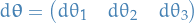
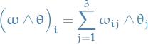
The first structure equations are

where the wedge product between the vectors are taken as
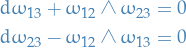
The second structure equations are

Definition of connection 1-forms and second structure equations only requires the existence of a moving frame and not a map .
The structure equations exist in the more general context of Riemannian geometry, where  is the Riemann curvature, which in general is non-vanishing. In our case it's zero because our moving frame is in
  .
.
Structure equations for surfaces
Notation
 are 1-forms
 are "connection" 1-forms
Adapted frames and the structure equations
A moving frame  for on is said to be adapted to the surface if
  .
.
I.e. it's adapted to the surface if we orient the basis such that  corresponds to the normal of the surface.
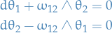
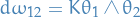
The first and second structure equations for a local surface wrt. to an adapted frame, give the structure equations for a surface:
First structure equations:
Symmetry equation:

Gauss equation:

Codazzi equations:
Notice how  has just vanished if you compared to in a moving frame, which comes from the fact that in an adapted moving frame we have .
The Gauss equation above is equivalent to
This shows that the Gauss curvature can be computed simply from a knowledge of  and
and  without reference to the local description of the surface .
Let be a local surface with the first fundamental form and  be the 1-forms on such that

Then there exists a unique adapted frame such that  and
and  .
.
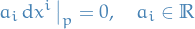
We say a 1-form is degenerate if wrt. any basis , the matrix representing the 1-form has  .
.
Two local surfaces and  are isometric if and only if
  .
.
Isometric surfaces have the same Gauss curvature. More specifically,
If  are two isometric surfaces, then

The Guass curvature is an instrinsic invariant of a surface!
The first fundamental form of a surface actually then turns out to determine the following properties:
- distance
- angles
- area
Geodesics
Notation
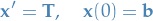
![$\mathbf{x}: [a, b] \to \mathbb{E}^n$](../../assets/latex/geometry_fd54d2659862f5acb5d8923d837a55e7851b62bf.png) which defines the map
which defines the map  , and has unit speed
  joining two points
Stuff
Consider a 1-parameter family of nearby curves

where 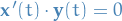 and
and 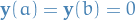 so that all curves in the family join
  to
to  . We refer to
  as a connecting vector.
It's very important that , because if has a component along  we could remove the shared component by reparametrising
  .
.
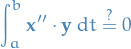
We say a unit speed curve as above has stationary length if the length of the nearby curves  satisfies
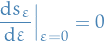
for all connecting vector  .
.
A unit speed curve in Euclidean space has stationary length if and only if it is the straight line joining the two points.
Let be a unit speed curve in Euclidean space. We then have to prove the following:
- is a straight line, then it has stationary length
- has stationary length then it's a straight line
Remember, stationary length is equivalent of
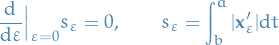
First, suppose that is in fact a straight line, then
Now, taking the square root and the derivative wrt.  we have

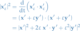
Remembering that is a unit-speed curve, i.e. , thus
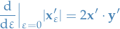
Now, substituting this into the expression for  , and observing that interchanging the integral wrt.
  and derivative wrt. is alright to do, we get
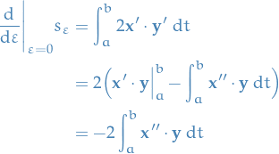
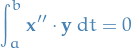
since by definition of connecting vectors. The final integral is zero if and only if  , which is equivalent of saying that is linear in and thus is a straigt line, concluding the first part of our proof.
Now, for the second part, we suppose that has stationary length
We again perform exactly the same computation and end up with the same integral as we got previously (since we did not use any of our assumptions until the very end), i.e.
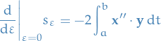
And since is assumed to have stationary length,
which is true if and only if  , hence by the same argument as above, is the straight line between the two points
  and
and  .
.
Notice the "calculus of variations" spirit of the proof! Marvelous, innit?!
Geodesics on surfaces
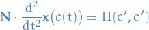
A unit-speed curve  lying in a surface is a geodesic if its acceleration is everywhere normal to the surface, that is,
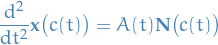
where is the unit normal to the surface and is some function along the curve.
This means that for a geodesic the acceleration in the direction tangent to the surface vanishes thus generalising the concept of a straight line in a plane.
You can see this from looking at the proof of stationary length in Euclidean space being equivalent to the curve being the straight line: in the final integral we have a dot-product between  and ,
and ,
But, all  defined in the definition of a connecting vector / nearby curves also lies on the surface, hence cannot have a component in the direction perpendicular to surface. Neither can since this is also on the surface, which implies also cannot have a component normal to the surface. Thus,

Finally implying
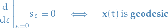
A curve lying in a surface has stationary length (among nearby curves on the surface joining the same endpoints) if and only if it's a geodesic.
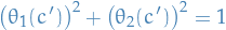
A curve lying in a surface is a geodesic if and only if, in an adapted moving frame it obeys the geodesic equations
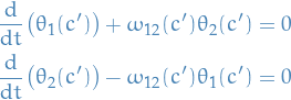
and the energy equation
Given a point on a surface and a unit tangent vector to the surface at , there exists a unique geodesic on the surface  for
for  (with sufficiently small), such that
  and
and  .
.
The geodesic equations only depend on the first fundamental form of a surface. Hence they are partof the intrinsic geometry of a surface and isometric surefaces have the same geodesics!
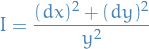
Two-dimensional hyperbolic space is the upper half plane
equipped with the first fundamental form given by
Integration over surfaces
Notation
 defines a local map , where we drop the bold-face notation due to not anymore using the Euclidean structure
 denotes the pull-back of
  by the map
Integration of 2-forms over surfaces
Let  define a local surface
Note we do not write the map defining the surface in bold here, to emphasise we are not going to use the Euclidean structure).
Let

be a 2-form on . We define the pull-back of by the map to be the 2-form on given by

IMPORTANT: where here  is the exterior derivative of
  , i.e.
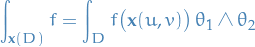
Let be a local surface and let be a 2-form on . We define the integral of over the local surface to be
So, we're defining the integral of the 2-form over the map as the integral over the pull-back of over the domain .
Why is this useful? It's useful because we can integrate some 2-form in the "target" manifold over the "input" domain .
Let be a k-dimensional oriented closed and bounded submanifold in with boundary  given the induced orientation and
  . Then
The Stokes' and divergence of vector calculus are the  and
and  special cases respectively.
Integration of functions over surfaces
For a local surface, we have

Hence, we obtain an alternate expression for the area
Thus the are depends only on , hence it's an intrinsic property of the surface.
For a local surface  with an adapted frame,

Let be a local surface and be a function.
Then the integral over over the surface is given by
In particular,
gives the are of the local surface. The 2-form  is called the area form.
Definitions
Words
- space-curves
- curves in
- plane curves
- curves in

- canonically
- "independent of the choice"
- rigid motion / euclidean motion
- motion which does not change the "structure", i.e. translation or rotation
Regular curves
A curve is regular if its velocity (or tangent) vector  .
.
The tangent line to a regular curve at  is the line
  .
.
A unit-speed curve  is biregular if
  , where
  denotes the curvature.
(Note that a unit-speed curve is necessarily regular.)
The principal normal along a unit-speed biregular curve is
The binormal vector field along is

The norm of the velocity
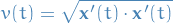
is the speed of th curve at .
A parametrisation of a regular curve s.t.  is called a unit-speed parametrisation.
Level set
The level set of a real-valued function of  variables is the set of the form

Arc-length
The arg-length of a regular curve  from to is
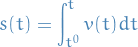
For a unit-speed parametrisation we have  , hence it is also called an arc-length parametrisation.
As we can see in the notes, there's a theorem which says that for any regular curve, there exists a reparametrisation of which is unit-speed.
Most reparametrisations are difficult to compute, and thus it's mostly used as a theoretical tool.
Example: Helix
The helix in is defined by
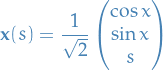
which is an arc-length parametrisation
Curvature
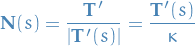
The unit tangent vector field along a regular curve is is
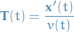
Thus, for a unit-speed curve it is simply  .
.
For a unit-speed curve the curvature  is defined by
Torsion
The torsion of a biregular unit-speed curve is defined by

or equivalently  .
.
The oscillating plane at a point on a curve is the plane spanned by  and . The torsion measure how fast the curve is twisting out of this plane.
Isometry
An isometry of is a map  given by

where is an orthogonal matrix and  is a fixed vector.
If  , so that is a rotation matrix, then the isometry is said to be Euclidean motion or a rigid motion.
If  the isometry is orientation-reversing.
By definition, an isometry preserves the Euclidean distance between two points  .
.
Tangent spaces
 we define the tangent space to at as the set of all derivative operators at , called tangent vectors at
and thus we have
in the notation we love so much.
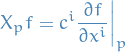
Vector fields are directional derivatives.
A vector field is defined by the tangent at each point for all in the domain of the vector field.
It's important to remember that these are curves which are parametrised arbitrarily, and thus describe any potential curve not just the you are "used" to seeing.
In words
- Tangent space of a manifold facilitiates the generalization of vectors from affine spaces to general manifolds
Tangent vector
There are different ways to view a tangent vector:
Physists view
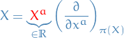
Basically considers the tangent vector as a directional derivative
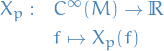
A tangent vector to at is determined by an n-tuple
for each choice of coordinates at , such that,  is the set of coordinates, we have
In your "normal" vector spaces we're used to thinking about direction and derivatives as two different concepts (which they are) which can exist independently of each other.
Now, in differential geometry, we only consider these concepts together ! That is, the direction is defined by the basis which the tangent vectors ("derivative" operators) defines.
"Geometric" view
This is a more "intuitive" way of looking at tangent vectors, which directly generalises the concept used in Euclidean space.
A (regular) curve in is a (smooth) map  , given by
where each  is a smooth function, such that its velocity
is non-vanishing,  , (as an element of ) for all
  . We say that a curve
  passes through if, say
  (without loss of generality one can always take the parameter value at to be 0).
 means a map from the open range
  to
to  , NOT a map which "takes two arguments", duh…
Let be a curve that passes through . There exists a unique  such that for any smooth function
There is a one-to-one correspondence between velocities of curves that pass through and tangent vectors in . By (standard) abuse of notation sometimes we denote  by the corresponding velocity
  .
.
Tangent vector of smooth curves
This approach is quite similar to the geometric view of tangent vectors described above, but I prefer this one.
As of right now, you should have a look at the section about Tangent space and manifolds, as I'm not entirely sure whether or not this can be confusing together with the different notation and all. Nonetheless, the other section is more interesting as it's talking about tangent vectors and general manifolds rather than the more "specific" cases we've been looking at above.
Let  be a smooth curve and
 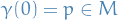 (wlog).
The tangent vector to curve  at is a linear map
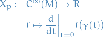
where
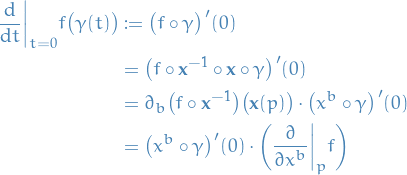
where  is a chart map.
Often denote  by
by  .
.
Tangent as the dual-space of the cotangent space
This section introduces the tanget space as the dual of the cotangent space. Furthermore, we construct the cotangent space in quite a "axiomatic" manner: defining the cotangent space as a quotient space of real-valued smooth functions on the manifold . It is almost an exact duplicate of the lecture notes provided by Prof. José Miguel Figueroa-O'Farrill in the course Differentiable Manifolds taught at University of Edinburgh in 2019.
- Notation
Zero-derivative vector subspace

- Stuff
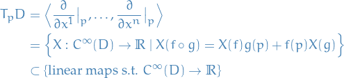
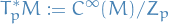
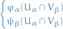
The cotangent space at some point
 is the quotient vector space
where
i.e. all those functions which have vanishing derivative when composed with the inverse of some chart map
 .
.
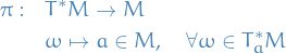
The derivative of
 at is the image of under the surjective linear map
which is simply the canonical map arising from the original space
 to the quotient space
  .
.
Observe that
 , and so we can indeed take the derivative.
 as defined in the definition of the cotangent space forms a vector subspace.
If
 is a smooth function in a neighborhood of , we can multiply by a some bump-function
  to construct .
For any choice of bump function
, agrees with in some neighborhood of . Therefore its derivative at is independent of the bump function chosen. Thus we can define the derivative at of functions which are only defined in a neighborhood of , e.g. the coordinate functions!
Let
be an n-dimensional manifold. Then
 is an n-dimensional vector space
- If
 is a coordinate chart around with local coordinates
  then
then  are a basis for .
 If
, then
If
then letting  means that
is a (locally defined) smooth function whose derivative vanish at
. This is seen by considering the composition with  :
:

where
 denotes the Euclidean coordinates, i.e.
 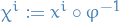 . This implies that
(since the partial derivative wrt.
"pass through ).
Therefore,
and hence
span .
Now we just need to show that
are also linearly independent. Suppose
Then the function
 has vanishing derivative at , and so
  has vanishing derivative at
  . But is a linear function and so the derivative at any point vanish if and only if it is the zero function. Therefore
  for all
  , and so are also linearly independent, and hence form a basis of
  .
.
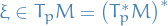
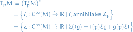
The tangent space
 at is the dual of the cotangent vector space. .
This is reasonable for finite-dimensional spaces since in these cases
 for vector space , i.e. dual of dual is original vector space.
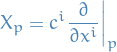
If
is the local coordinate at and is a basis of , the canonical basis for is denoted
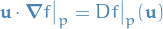
To relate the tangent space to a more intuitive notion, we introduce the directional derivative.
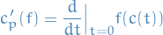
A directional derivative at
is a linear map
s.t.

Observe that if
 it defines a linear map
and from the formula for
 ,
,
Therefore
is a directional derivative at
.
All tangent vectors are of this form.
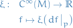
An example of a directional derivative is if
 , then for any tangent direction
  to at
to at  we can define the derivative of at along to be the real number
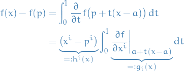
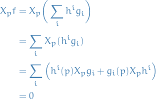
Let
be a directional derivative at and let  . Then

Use a coordinate chart near
. By the FTC,
Using a bump function we can extend
 and
and  from a neighborhood of to .
Notice that
 and if
  then
then  as well. Therefore

By the Leibniz rule,

and by linearity,
 . Therefore
Therefore
kills and descends to a linear map  , i.e.

Therefore, as a result of the above lemma, we get

we can also write
Relative to local coordinates,
and
Tangent bundle
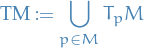
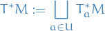
The tangent bundle of a differential manifold is a manifold  , which assembles all the tangent vectors in . As a set it's given by the disjoint union of the tangent spaces of , i.e.

Thus, an element in can be thought of as a pair  , where is a point in the manifold and
  is a tangent vector to at the point .
Let be a smooth manifold. Then the tangent bundle is the set
and further we define the bundle projection:
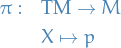
where is the point for which  . This gives us a set bundle; now we just have to show that the fibres are indeed isomorphic, and thus we've obtained a fibre bundle.
Idea: construct a smooth atlas on  from a given smooth atlas on .
- Take some chart

Construct

where we define
 as
as
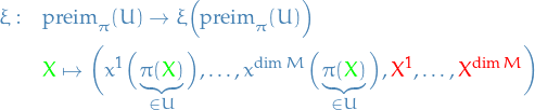
where
- First
 coordinates we observe is projecting the tangent at some point onto the point itself , i.e.
 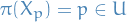 (we don't write in the above because we can do this for any point in the manifold)
 Second
coordinates account of the direction and magnitude of the tangent  , i.e. we choose the coefficients of in the tangent space at that point!
- First
Finally we need to ensure that this map
is indeed smooth :
We start by considering the total space, which is the space of all sections  , i.e.

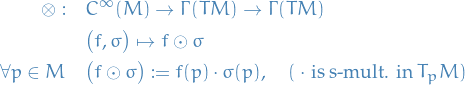
equipped with the two operations:
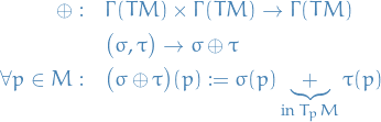
and multiplication:
Cotangent bundle
Let be n-dimensional and let
denote the disjoint union of all the cotangent spaces of .
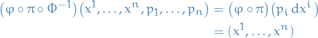
If is a chart of , then the map
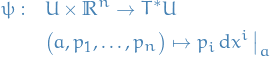
defines a bijection, and allows us to define

It then follows that  is a bjection from
  to an open subsets of
  , hence
  defines a chart of
  . In this way we can bring the charts of up to , thus is a manifold.
 be an
be an 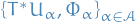 is an atlas of
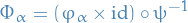
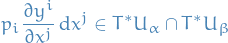
Since 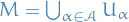 we have that
  . Therefore we only need to check that indeed the transition maps

First observe that

which is an open subset of . So the transition map is open. To see smoothness, let  be local coordinates of
  and
and  be local coordinates of
  . Then

and
so
Therefore
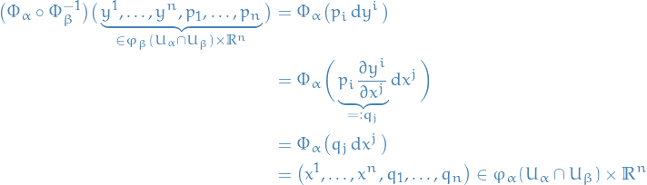
Since  is a diffeomorphism
  is smooth in the first components. Furthermore,
 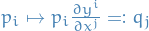 is smooth since the derivative of smooth functions are smooth and
  depends linearly on
  .
.
Hence, is smooth for all  , and so
  defines an atlas for .
Let
i.e. in local coords we have 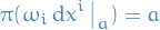 .
.
 is smooth.
being "smooth" means that

is a smooth map.
Let be local coordinates of . Then
since 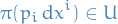 . More concretely,

Hence,

which is clearly smooth since are all smooth maps.
is Hausdorff and second countable.
Second-countability follows directly from the fact that  is second-countable, and so is second-countable.
In what follows we are considering  as points, i.e.
  for some
  .
.
Let  and
and  , then we have the following two cases:
 : since is Hausdorff, there exists two sets
  such that
  , and so we're good.
 : we have chart
  , and so
  is homeomorphic to some subset of . is Hausdorff, therefore
  such that
  and
and  .
.
Hence is also Hausdorff.
In the above we are talking about open subsets of but as we have seen before, since chart  induces chart
  , any set
  open is equivalent to saying that the intersection
  is open for
  . This in turn means that there exist some such that
  , therefore we can equivalently consider this open set .
Dual space
Let be a vectorspace over . Then the dual space of denoted as , is given by

Properties
Dual Basis
Honestly, "automatically" is a bit weird. What is actually happening as follows:
Suppose that we have a basis in defined by the set of vectors  . then we can construct a basis in the dual space , called the dual basis. This dual basis is defined by the set
  of linear functions / 1-forms on , defined by the relation

for any choice of coefficients  in the field we're working in (which is usally ).
In particular, letting each of these coefficients be equal to 1 and the rest equal zero, we get the following set of equations
which defines a basis.
If  is a basis for , we automatically get a dual basis
  for , defined by
If  (is finite), then
Dual of the dual
If

Map between duals
If  in a linear map between (dual) vector spaces
  get canonically a dual map :

1-forms
Aight, so this is the proper definition of a one-form.
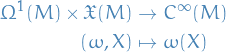
A (differential) one-form is a smooth section  on the cotangent bundle, i.e. satisfying
We denote the space of one-forms as  .
.
is a  .x
.x
Let
- be a chart of with local coordinates
- be a chart of as defined in def:cotangent-bundle
Define
To see that
 we need the map

to be smooth. Writing the the map out explicitly, we have

where
 (i.e. it's really just ), which is smooth by smoothness of
 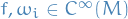 .
.
Define
Again we require smoothness of the corresponding composition with the charts:
which again is smooth since
 are smooth sections, i.e.
  .
.
Hence, is closed under (scalar)  and addition, i.e. defines a module.
 : follows directly from the fact that both and
  are
are  , and
, and  .
.Non-degenerate: suppose
 is non-zero and

Then either
 or
or  forall . The non-degeneracy for
  follows by an almost identical argument.
[DEPRECATED] Old definition
A 1-form at is a linear map  . This means, for all
  and
and  ,
,

1-forms is equivalent to linear functionals
The set of 1-forms at , denoted by , is called the dual vector space of
We define 1-forms  at each by their action on the basis
  :
:
Or equivalently,  are defined by their action on an arbitrary tangent vector
  :
:

Differential 1-form
A differential 1-form on is a smooth map which assigns to each a 1-form in ; it can be written as:
where  are smooth functions.
Line integrals
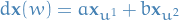
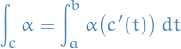
Let ![$c : [a, b] \to D$](../../assets/latex/geometry_5e5e47eb13f6fa87443f659e0904306b92113ff6.png) be a curve (the end points are included to ensure the integrals exist) and on the 1-form on . The integral of over the curve is
be a curve (the end points are included to ensure the integrals exist) and on the 1-form on . The integral of over the curve is
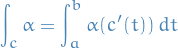
where  is the tangent vector field to the curve.
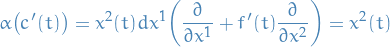
Working in coordinates, the result of applying the 1-form on gives the expression
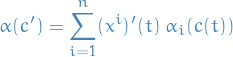
i.e. the derivative of wrt. times the evaluation of  at , where denotes the evaluation of along .
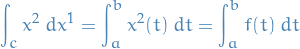
![\begin{equation*}
c(t) = \big( t, f(t) \big), \qquad t \in [a, b]
\end{equation*}](../../assets/latex/geometry_4334797f3364c71ae763474faffb8b84ca6da38c.png)
 is just the usual integral
  .
.

 .
.
k-form
A 2-form at is a map  which is linear in each argument and alternating

More generally, a k-form at is a map of vectors in to which is multilinear (linear in each argument) and alternating (changes sign under a swap of any two arguments).
And even more general, on the vector space with  , a k-form (
 ) is a
  tensor that is anti-symmetric, e.g. for a 2-form

In the case of a k-form, if  , where
  , then
  are top forms, both non-vanishing:

i.e. any two top-forms are equal up to a constant factor.
Further, the definition of a volume on some d-dimensional vector space, completely depends on your choice of top-form.
Wedge product
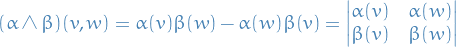
The wedge product or exterior product  of 1-forms and
  is a 2-form defined by the following bilinear (linear in both arguments) and alternating map
More generally, the wedge product of 1-forms,  can be defined as a map acting on vectors
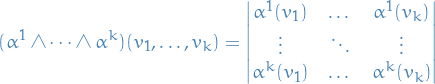
From the properties of the determinant it follows that the resulting map is linear in each vector sperarately an changes sign if any pair of vectors is exchanged (this corresponds to exchanging two columns in the determinant). Hence it defines a k-form.
Wedge product between different forms
We extend  linearly in order to define the wedge product of a -form and an
  -form . Explicitly,

Here the sum is happening over all multi-indices and  with
with  and
and  .
.
Now two things can happen:
 , in which case
  since there will be a repeated index
 , in which chase
  , for some muli-index K of length
  . The sign is due to having to reorder them to be increasing.
Therefore, the wedge product defines a (bilinear) map

Multi-index
Useful as more "compact" notation.
By a multi-index of length we shall mean an increasing sequence  of integers
  . We will write

The set of k-forms at is a vector space of dimension  for
for  with basis
  .
.
Here denotes the maximum number of dimensions. So we're just saying that we're taking the wedge-product between some indicies of the 1-forms we're considering.
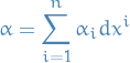
Differential k-form
A differential k-form or a differential form of degree k on is a smooth map which assigns to each a k-form at ; it can be written as

where  are smooth functions, and the sum happens over all multi-indices with .
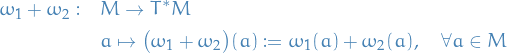
Given two differential k-forms  and a function the differential k-forms
  and
and  are
are

The set of k-forms on is denoted  .
.
By convention, a zero-form is a function. If  then
then  (for every form has a repeated index).
To make the notation used a bit more apparent, we can expand for  in for a vector-space in , i.e.
  , defined above as follows:

where we've used the fact that  . and just combined the "common" wedge-products.
It's very important to remember that the here represents a 0-form / smooth function.
The actual definition of is as a sum of all possible
. and just combined the "common" wedge-products.
It's very important to remember that the here represents a 0-form / smooth function.
The actual definition of is as a sum of all possible  but the above definition is just encoding the fact that
  .
.
A form  is said to be closed if
  .
.
A form  is said to be exact if

for some  .
.
 , then it is also
 Exterior derivative
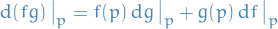
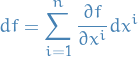
Let (i.e. it's a 0-form), and define
where  denotes the exterior derivative (or the "differential") of .
Then is a one-form, i.e.

First recall that for a chart with local coordinates ,
 is smooth:
Let
is smooth:
Let  be a chart defined as in def:cotangent-bundle, then the map is smooth iff

is smooth. Writing out this map we simply have
REMINDER: recall what
 actually means.
where
 denotes the partial derivative wrt. the i-th component of the map.
 is clear
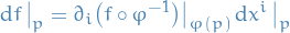
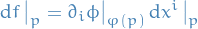
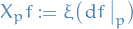
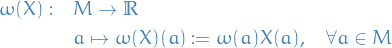
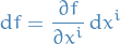
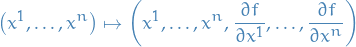
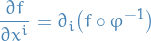
Given a smooth function on , its exterior derivative (or differential) is the 1-form  defined by

for any vector field  . Equivalently
Let  be a smooth function, i.e.
  .
.
As it turns out, in this particular case, the push-forward of , denoted  is equivalent to the exterior derivative!
If 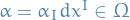 , then its exterior derivative
  is
is

where  denotes the exterior derivative of the function
  (which we defined earlier).
More explicitly, take the example of the exterior derivative of a 1-form, i.e.  :
:
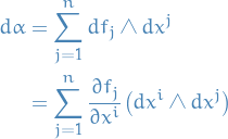
from the the definition of where is a function (0-form), and 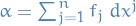 .
.
Theorems
The exterior derivative  is a linear map satisfying the following properites
 obeys the graded derivation property, for any

 for any , or more compactly,
Example problems
Handin 2
Let ![$c : [0, 2 \pi] \to \mathbb{R}^3$](../../assets/latex/geometry_05ac517ec743fcf34e663993a224a289b0158f45.png) be the helix
be the helix 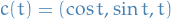 and consider the 1-form on

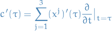
Find the tangent
at each point along curve. Hence evaluate the line integral of the 1-form along the curve .
 1
1
Hence the integral is
The tangent plane at some point
 along the curve for a specified
  is given by
 2
2
which in this case is equivalent of
3
Concluding the first part of the claim.
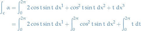
For the integral, we know that
4
for the boundaries
 and
and  .
Computing
.
Computing  we get
 5
5
 6
6
- Show that . Now find a smooth function
 such that
  . Hence evaluate the above line integral without explicit integration.
Integration in Rn
The standard orientation (which we always assume) is defined by

Coordinates  (an ordered set) are said to be oriented on if and only if
  is a positive multiple of
  for all
  .
.
Observe that this induces an orientation on , since we simply apply to the coordinates , thus returning a  or
or  dependening on whether or not the surface is oriented.
Let be oriented coordinates for . Let be smooth functions on . Then
where the factor on the RHS is hte Jacobian of the coordinate transformation (i.e. the determinant of the matrix whose  component is
  .
.
Let be oriented coordinates on and write

Then the integral of  over is defined by
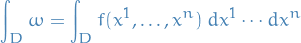
where the RHS is now the usual multi-integral of several variable caculus (provided it exists).
Topological space
A topological space may be defined as a set of points, along with a set of neighbourhoods for each point, satisfying a set of axioms relating points and neighbourhoods.
Or more rigorously, let be a set. A topology on is a collection  of subsets of , called open subsets, satisfying:
- and
 are open
 - The union of any family of open subsets is open
- The intersection of any finite family of open subsets is open
A topological space is then a pair  consisting of a set together with a topology on .
The definition of a topological space relies only upon set theory and is the most general notion of mathematical space that allows for the definition of concepts such as:
- continuity
- connectedness
- convergence
A topology is a way of constructing a set of subsets of such that theese subsets are open and satisfy the properties described above.
Atlases & coordinate charts
A chart for a topological space (also called a coordinate chart, coordinate patch, coordinate map, or local frame ) is a homeomorphism  , where
  is an open subset of . The chart is traditionally denoted as the ordered pair
  .
.
An atlas for a topological space is a collection  , indexed by the set , of charts on s.t.
  .
.
If the codomain of each chart is the n-dimensional Euclidean space, then is said to be n-dimensional manifold.
Two atlases  and
and  on are compatible if their union is also an atlas.
So we need to check the following properties:
The following are open in
for all  and all
 and
and  are
are  for all and all .
Compatibility of atlases define a equivalence relation of atlases.
A differentiable structure on is an equivalence class of compatible atlases.
Often one defines differentiable structure with a "maximal atlas" instead of an equivalence class. The "maximal atlas" is obtained by simply taking the union of all atlases in the equivalence class.
A transition map is a composition of one chart with the inverse of another chart, which defines a homeomorphism of an open subset of the onto another open subset of the ..
Suppose we have the following two charts on some manifold
such that

The transition map is defined
where we've used the notation
to denote that the function is restricted to the domain 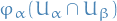 , i.e. the statement is only true on that domain.
A differentiable manifold is a topological manifold equipped with an equivalence class of atlases whose transition map are all differentiable.
More generally, a manifold is a topological manifold for which all the transition maps are all k-times differentiable.
A smooth manifold or manifold is a differentiable manifold for which all the transition map are smooth.
To prove is a smooth manifold if suffices to find one atlas due to the compatibility of atlases being an equivalence relation.
A complex manifold is a topological space modeled on the Euclidean space over the complex field and for which all the transition maps are holomorphic.
When talking about "some-property-manifold", it's important to remember that the "some-property" part is specifying properties of the atlas which we have equipped the manifold with.
is smooth if for any chart , the function

is smooth.
Observe that if  is smooth for a chart
  , then we can transition between patches to get a smooth map everywhere.
Let  with
with  and
and  .
.
Then is smooth if for every and charts with  and
and  with
with  , we have
That is,

where denotes smooth functions on  .
.
Examples
Real projective space
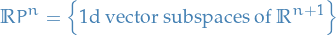
If  spans a 1d subspace (up to multiplication by real numbers). So, for each
 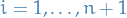 , we let

Then
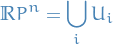
and we further let
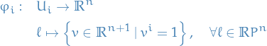
Real with global charts
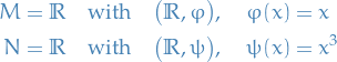
then

is not diff. at  .
.
 as a manifold (which can be seen by noticing that the identity map is not ).
But and are diffeomorphic:
Then
is and invertible with inverse.
Manifolds
A topological space that locally resembles the Euclidean space near each point.
More precisely, each n-dimensional manifold has a neighbourhood that is homomorphic to the Euclidean space of dimension .
Immersed and embedded submanifolds
An immersed submanifold in a manifold is a subset  with a structure of a manifold (not necessarily the one inherited from !) such that the inclusion map
  is an immersion.
Note that the manifold structure on s part of the data, thus, in general, it is not unique.
Note that for any point  , the tangent space to is naturally a subspace of the tangent space to , i.e.
  .
.
An embedded submanifold is an immersed manifold such that the inclusion map is a homeomorphism, i.e. is an embedding.
In this case the smooth structure on is uniquely determined by the smooth structure on .
In words, the inclusion map being a homeomorphism means the manifold topology of agrees with the subspace topology of  .
.
Let  be smooth. Then
  if
if  is surjective on
  , i.e.

or equiv,

then we say that is a regular value (for ).
Let
- be a smooth map and
 and
and - be a regular value (for )
Then  is an embedded submanifold of of dimension , and
From Rank-Nullity theorem applied to , using the fact that  since it's surjective on
  .
.
Let
be an embedding. Then  is the constant map
  .
.

The rest follows from the Rank-Nullity theorem.
Examples
- Figure 8 loop in
It is immersed via the map

- This immersion of
 in fails to be an embedding at the crossing point in the middle of the figure 8 (though the map itself is indeed injective)
 - Thus, is not homeomorphic to its image in the subspace / induced topology.
Riemannian manifold
A (smooth) Riemannian manifold or (smooth) Riemannian space  is a real smooth manifold equipped with an inner product
  on the tangent space at each point that varies smoothly from point to point in the sense that if and
  are vector fields on the space , then:
is a smooth function .
The family of inner products is called a Riemannian metric (tensor).
The metric "locally looks linear":)
The Riemannian metric (tensor) makes it possible to define various geometric notions on Riemannian manifold, such as:
- angles
- lengths of curves
- areas (or volumes)
- curvature
- gradients of functions and divergence of vector fields
Euclidean space is a subset of Riemannian manifold
Resolving some questions
- Why do we need to map the point to two vector-spaces
 before applying the metric ?
Because it's the tangent space which is equipped with the metric , not the manifold itself, and since vector spaces are defined by a basis in we need to map into this space before applying .
before applying the metric ?
Because it's the tangent space which is equipped with the metric , not the manifold itself, and since vector spaces are defined by a basis in we need to map into this space before applying . - What do we really mean by the map
 being smooth ?
This means that this maps varies smoothly wrt. the point .
being smooth ?
This means that this maps varies smoothly wrt. the point . - The Riemannian metric is dependent on , why is that?
Same reason as the first question: the inner product is equipped on the tangent space, not the manifold itself, and since we have a different tangent space at each point , the inner product itself depends on the point chosen.
Differential manifold
Homeomorphism
A homeomorphism or topological isomorphism is a continuous function between topological spaces that has a continuous inverse function.
Diffeomorphism
A diffeomorphism is an isomorphism of smooth manifolds. It is an invertible function that maps one differentiable manifold to another such that both the function and its inverse are smooth.
That is, a smooth with a smooth inverse  .
.
It's worth noting that the term diffeomorphism is also sometimes used to only mean once-differentiable rather than smooth!
Isometric
An isometry or isometric map is a distance-preserving transformation between metric-spaces, usually assumed to be bijective.
Algebra
A K-vector space  equipped by a product, i.e. a bilinear map

is called an algebra 
Example: Algebra over differentiable functions
On some manifold , we have the vector-space  which is a -vector space, and we define the product
  as
as

by the map, for some  ,
,
where and the product on the RHS is just the s-multiplication in .
Equations / Theorems
Frenet-Serret frame
The vector fields  along a biregular curve are an orthonormal basis for for each
  .
.
This is called the Frenet-Serret frame of .
By definition of the unit tangent,  . Differentiate this wrt. to find
  . Thus, the principal normal satisfies and
 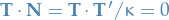 .
.
By definition of the binormal we also have  and
and  . Hence,
  form an orthonormal basis.
Structure equations
Let be a unit-speed biregular curve in . The Frenet-Serret frame  along satisfies:
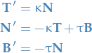
These are called the structure equations for unit-speed space curve, or sometimes the "Frenet-Serret equations".
See p. 9 in the notes for a proof.
For a general parametrisation of a biregular space curve the structure equations become
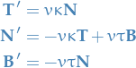
where is the speed of the curve.
Extras
A biregular curve is a plane curve if and only if  everywhere.
If lies in a place, then and are tangent to the plane and so  must be a unit normal to this plane and hence constant.
The structure equations then imply .
The curvature and torsion of a biregular space curve in any parametrisation can be computed by

Matrix formulation
The structure equations can also be expressed in matrix form:
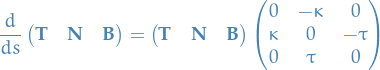
By ODE theory, for given and  and initial conditions

there exists a unique solution

to the ODE system, and hence it must conicide with the Frenet-Serret frame.
There is then a unique curve satisfying
Equivalence problem
The equivalence problem is the problem of classifying all curves up to rigid motions.
Uniqueness of biregular curve
Let and be given, with everywhere positive. Then there exists a unique unit-speed biregular curve with these as curvature and torsion such that  and
and  is any fixed oriented orthonormal basis in .
Fundamental Theorem of Curves
If two biregular space curves have the same curvature and torsion  then they differ at most by a Euclidean motion.
Tangent spaces
Orthogonality
Change of basis
Suppose we have two different bases for a space:

we have the following relationship
and for the dual-space
Implicit Function Theorem
Let  , where is the base and is the "extra" dimension.
Let be an open subset of  , and let
  denote standard coordinates in .
Suppose  is smooth,
  with
with  and
and  , and
, and
If the  matrix

is invertible, then there exists neighbourhoods  of and
  of and a smooth function

such that:

is the graph of  .
.
Or, equivalently, such that

I like to view it like this:
Suppose we have some dimensional space, and we split it up into two subspaces of dimension  such that

Then, using Implicit Function Theorem, we can simply check the invertibility of the Jacobian of , as described in the theorem, to find out if there exists a function  where and .
Where , where  , is a map "projecting" some neighbourhood / open set of to
  .
.
Example
Consider  and
and  . Ket
. Ket
Then,

Consider  and
and  , and
, and 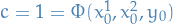 .
.
Thus,
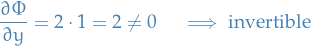
Thus, in the neighbourhood of  in we can consider the level set
  and locally solve as a function of
  , i.e. there exists a function such that
  .
.
Inverse Function Theorem
Let be a differentiable map, i.e.  . If
. If
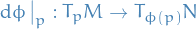
is a linear isomorphism at a point in , then there exists an open neighborhood  such that
is a diffeomorphism.
Note that this implies that and must have the same dimension at .
If the above holds , then is a local diffeomorphism.
Gauss-Bonnet
Let be an oriented closed and bounded surface with no boundary. Then
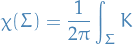
where  is the Euler characteristic of the surface , defined as
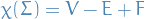
where denotes the vertices,  the edges, and the faces obtained by dissecting the surface into polygons (this turns out to be independent of choice of dissection).
Change of basis
Notation
- Einstein summation notation
- is a K-vector space, i.e. vector space over some field

 denotes the b-th basis-vector of some basis in
  means isomorphic to
 denotes a tensor of order
Stuff
Suppose we have two different bases in some K-vector space :

Now, how does the this affect the 1-forms / covectors (contra-variant) change?
k-forms / covectors
Let be a covector:

where  denotes the m-th new basis!

is true since is a linear map by definition.
vectors

where the only thing which might seem a bit weird is the
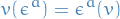
which relies on

where

i.e. is isomorphic to the the dual of the dual space, which is only true for a finite basis!
Apparently this can be shown using a "constructive proof", i.e. you build up the notation mentioned above and then show that it does indeed define an isomorphism between the vector-space and the dual of the dual space.
Determinants
Notation
Stuff
Problem with matrix-representation
A matrix is a  tensor, and we can thus write it as
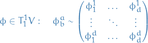
where  means that we can write out an exhaustive representation of all the and entries in such a way (in this case a matrix).
Also, it turns out that we can write a bilinear map as
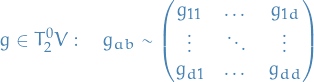
See?! We can represent both as a matrix, but the way the change with the basis are completely different!
The usual matrix representation that we're used to (the one with the normal matrix-multiplication, etc.) is the  tensor, and it's an endomorphism on , i.e. homomorphism which takes a vector to a vector.
Definition
Let  . Then
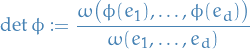
for some volume form / top-form , and for some basis  of , i.e. it's completely independent from the choice of basis and top-form.
Due to the top-forms being equal up to some constant, we see that any constant in the above expression would cancel.
Tangent space and manifolds
Notation
 , that is a linear map from the manifold and , often called a chart map (as it is related to a chart
  )
)
 is a smooth curve, i.e. a smooth mapping taking in a single parameter and mapping it to a point on the manifold
  is the partial derivative, which at each point
  (since ) for some function
  we take the partial derivative of wrt. a-th entry of the Cartesian product
  (n times)
Stuff
We define a new symbol
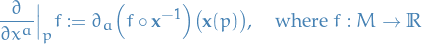
that is
Why is this all necessary? It's pretty neat because we're first using the chart-map to map the point to Euclidean space.
Then, the composite function 
The tangent space is an n-dimensional (real) vector space.
Addition structure:
Consider two curves  in s.t.
with tangent vectors and  .
We let
.
We let

Need to show that  curve
curve  , s.t.

Let  be a chart,
  . Then we define by
![\begin{equation*}
\phi \big( \nu(t) \big) = \alpha \big[ \phi \big( \gamma(t) \big) - \phi(p) \big] + \beta \big[ \phi \big( \mu(t) \big) - \phi(p) \big] + \phi(p)
\end{equation*}](../../assets/latex/geometry_1790b756db4bc4eee38a22ac9b31deb45a883ac6.png)
so  and
and
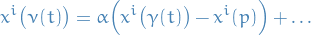
where are the components of the chart.
Tangent vector to at :
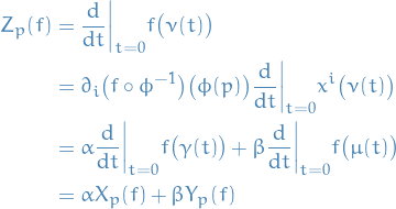
where we have used the fact that
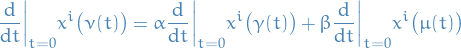
N-dimensional follows from Theorem thm:tangent-vectors-form-a-basis: They form the basis
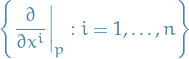
thus  .
.
Construting a basis
From above, we can construct vectors
which are the tangent vectors to the chart-induced curves  .
.
Any ca be written as
where we're using Einstein summation and  refers to the s-multiplication of a in the vector space.
Further,
form a basis for  .
.
 ,
,  is a smooth curve through

Then the map  , which is the tangent vector of the curve at point given by
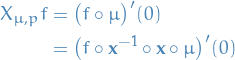
Then by the chain rule, we have:
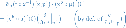
where we've used the fact that  is just a real number, allowing us to move it to the front.
Hence, for any smooth curve in at some point we can "generate" the tangent of this curve at point from the set
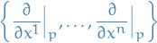
which we say to be a generating system of .
Now, all we need to prove is that they are also linearly independent, that is
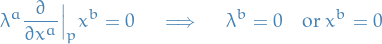
This is just the definition of basis, that if a vector is zero in this basis, then either all the coefficients are zero or the vector itself is the zero-vector.
One really, really important thing to notice in this proof is the usage of
where we just "insert" the  since itself is just an identity operation, but which allows us to "work" in Euclidean space by mapping the point in the manifold to the Euclidean space, and then mapping it back to the manifold for to finally act on it!
Push-forward and pullback
Let be a smooth map between smooth manifolds and .
Then the push-forward  at the point is the linear map
which defines the map

as
where:
 is a smooth function
- Elements in and
 define maps of functions, hence we need to apply it to some function to define it's operation
A couple of remarks:
- defined as above, is the only linear map from to
 one can actually define!
 - is often referred to as the derivative of at the point
- The tangent vector
 of the curve at the point in the manifold is pushed forward to the tangent vector of the curve
  at the point
  in the manifold ; i.e. for a curve we map the tangent vector at some point to the tangent vector of the "new" curve in the target manifold at the resulting point
- Or, pull-back (on functions) the curve by composition
 , and then let the tangent act on it
- Or, pull-back (on functions) the curve by composition
Let be a smooth map between smooth manifolds and .
Then the pull-back  of at the point
  is the linear map
i.e. a linear map from the cotangent space at the target TO the cotagent space of the originating manifold at point !
We define the map
as, acting on ,
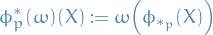
which is linear since and are linear, where is the push-forward.
Let
- be a smooth map
- , i.e. s.t.
Then

We need to show that  is indeed smooth.
Let
 be a chart in (with ) and
  be a local chart in (with
  )
)
Then in we can write  and
and  with
with  and
and  . Since
  , we have
  , therefore it's sufficient to consider how
  acts on a basis vector of
  , e.g.
  :
:
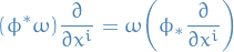
Recall that
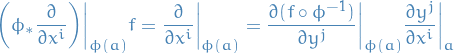
since  are the local coords of
  , which means
  can act on
  ; observe that
  . Therefore, going back to our original expression for :
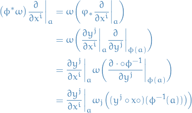

Equivalence with Jacobian in some chart
Let be a smooth math between manifolds.
Relative to local coordinates near and  near
near
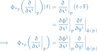
Comments on push-forward and exterior derivative
First I was introduced to the exterior derivative in the Geomtry course I was doing, and afterwards I was, through the lectures by Schuller, introduced to the concept of the push-forward, and the pull-back defined using the push-forward. Afterwards, in certain cotexts (e.g. in Geometry they defined the pull-back of a 2-form on  involving the exterior derivative), I kept thinking "Hmm, there seems to be some connection between the exterior derivative and the push-forward!
Then I read this stachexchange answer, where you'll find the following snippet:
Except in one special situation (described below), there is essentially no relationship between the exterior derivative of a differential form and the differential (or pushforward) of a smooth map between manifolds, other than the facts that they are both computed locally by taking derivatives and are both commonly denoted by the symbol
And the special case he's referring to is; when the function is a smooth map , where the two are equivalent.
Immersion, submersion and embedding
A submersion is a differentiable map between differential manifolds whose differential is surjective everywhere.
Let and be differentiable manifolds and be a differentiable map between them. The map is a submersion at the point if its differential

is a surjective linear map.
Let  be a smooth map on manifolds to .
We say is an immersion if and only if the derivative / push-forward is injective for each point , or equivalently  .
.
Remember the push-forward is a map from the tangent space of at point to the tangent space of at :  .
We do NOT require the map itself to be injective!
.
We do NOT require the map itself to be injective!
Let be a smooth map on manifolds and .
We say is an embedding of in if and only if:
- is an immersion
 , where
  means a homeomorphism / topological isomorphism
To summarize: A smooth map is called a
- submersion if
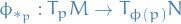 is surjective for for all (so
- immersion if is injective for all (so
 )
) - embedding if is an immersion and if the manifold topology of agrees with the subspace topology of
Any smooth manifold can be:
- embedded in

- immersed in

Where  .
.
This is of course "worst-case scenarios", i.e. there exists manifolds which can be embedded / immersed in lower-dimensional manifolds than the rules mentioned here.
There exists even stronger / better lower bounds for a lot of target manifolds, which requires slightly more restrictions on the manifold.
Let and me differentiable manifolds. A function

is a local diffeomorphism, if, for each point  , there exists an open set such that
  , and the image
  is open and

is a diffeomorphism.
A local diffeomorphism is then a special case of an immersion from to , where the image of under locally has the differentiable structure of a submanifold of .
Example: 2D Klein bottle in 3D
The klein bottle is a 2D surface, as we can see below:

But due to the self-intersecting nature of the Klein bottle, it is not a manifold when it "sits" in . Nonetheless, the mapping of the Klein bottle as shown in the picture, does in fact have a injective puh-forward! That is, we can injectively map each tangent vector at a point in such a manner that no two tangent vectors are mapped to the same tangent vector on the Klein bottle 2D surface in .
Hence, the Klein bottle can be immersed in but NOT embedded, as "predicted" by Whitney Theorem. And the same theorem tells us that we can in fact embed the Klein bottle in  .
.
Tensor Fields and Modules
Notation
 where denotes the tangent bundle of the manifold .
 is taking the Cartesian product and equipping it with addition
Homomorphisms

where
 refers to the fact that if
  and
and  we have
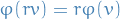
- Let
 be a (p, q)-tensor, then
 Symmetric summation
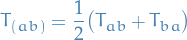
Anti-symmetric summation
![\begin{equation*}
T_{[a b]} = \frac{1}{2} \Big( T_{ab} - T_{ba} \Big)
\end{equation*}](../../assets/latex/geometry_2a84947d1db2b8686172fc0fe267c6e90c544c3b.png)
Vertical bars denote arguments which are excluded
![\begin{equation*}
\begin{split}
T_{(a |b| c)} &= \frac{1}{2} \Big( T_{abc} - T_{cba} \Big) \\
T_{[a |bc| d]} &= \frac{1}{2} \Big( T_{abcd} - T_{dbca} \Big)
\end{split}
\end{equation*}](../../assets/latex/geometry_7d28d1f486a5c63aca107bec80f61a27cc1a1833.png)
Stuff
Let
- be a smooth manifold
- be it's tangent bundle:

where
is smooth
A vector field is a smooth section of , i.e.
 is smooth
 is smooth
Informally, a vector field on a manifold can be defined as a function that inputs a point and outputs an element of the tangent space  . Equivalently, a vector field is a section of the tangent bundle.
Defined as a function on , a vector field  is smooth if
  are all smooth functions of .
Let and be a vector field on .
The function
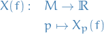
is smooth if and only if is smooth.
If chart  are smooth because
  is on the chart.
Conversely, if  , we choose
  , thus
  is smooth.
Module
We say  is a R-module,
  being a ring, if
satisfying

Thus, we can view it as a "vector space" over a ring, but because it behaves wildly different from a vector space over a field, we give this space a special name: .
Important: denotes a module here, NOT manifold as usual.
If is a division ring, then has a basis.
This is not a  but simply says that we guarantee the existence of a basis if is a division ring.
First we require the Axiom of Choice, in the incarnation of Zorn's lemma, which is just the Axiom of Choice restated, given that we already have all the other axioms of Zermelo-Fraenkel set theory.
Zorn's Lemma: A partially ordered set  whose every totally ordered subset
  has an upper bound in contains a maximal element.
where:
- partially ordered
Every module over a divison ring has a basis
Notation
- denotes the division ring
Theorem
Every module over a division ring has a basis.
Let
 be a generating system of , i.e.

Observe that
, the generating system, always exists since we can simply have 
Define a partially ordered set
 by
by

where
 denotes the powerset of .
We partially order it by inclusion:
denotes the powerset of .
We partially order it by inclusion:

i.e. if a set is a subset of another, then the it's smaller than the other subset.
Let
be any totally ordered subset of , then

and it is a lin. indep. subset of
.
Thus, by Zorn's Lemma, has a maximal element, one of which we call . By construction, is a maximal lin. indep. subset of .
Claim:
 Proof: Let
  . Since is maximal lin. indep. subset, we have
  is linearly dependent. That is,

and not all of
 , vanish, i.e.
  .
Now it is clear that
.
Now it is clear that  , because

but this is a contradiction to
 being linearly independent, as assumed previously.
Hence we consider ; then, since
being linearly independent, as assumed previously.
Hence we consider ; then, since  (remembering that is a division ring)

Thus, if we multiply the equation above with the inverse of
, we get
for the finite subsets
 of B. Thus,
Hence, we have existence of a linear indepndent subset of
which also spans .
As we see above, here we're making use of the fact that is a division ring, when we're using the inverse of  .
.
Observe that  is not a division ring, hence
  consider as a module is not guaranteed to have a basis.
Definition of can be found here.

Terminology
A module over a ring is called free if it has a basis.
Examples:
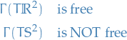
A module  over a ring is called projective if it is a directed summand of a free R-module :

where  is the R-module.
Remark: free projective
Theorems

is a finitely projective module  .
.
From this have the following corollary:
where is the module and is a free module.
Thus, "quantifies" how much fails to have a basis, since is how much we have to add to to make it free.
Let  be finitely generated projective modules over a commutative ring .
Then,
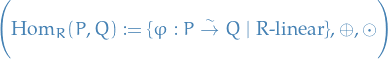
is again a finitely generated projective module.
This falls out of the commutativity of the ring .
In particular:
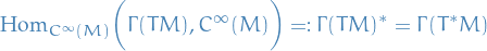
where the equality  can be shown (but we haven't done that here).
Finally, this gives us the "standard textbook definition" of a tensor-field:
A  tensor field on a smooth manifold is a multilinear map

We can then view
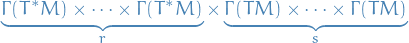
as the space of all tensor-fields on , which again, forms a module!
Hence, we when we talk about the mapping (see def:tensor-field for def) being multilinear, of course it must be multilinear to the underlying ring-structure of the module, i.e. multilinear!
Some textbooks give the above definition, and then note that is not linear, but linear, and that this needs to be checked. But because we're aware of the commutative ring that "pops out" we know that of course it has to be multilinear wrt. the underlying ring-structure, which in this case .
Metric tensor
A metric gensor on is a  over s.t.
symmetric:

non-degenerate:

Unlike an inner product, a metric tensor does NOT have to be positive-definite!
A standard example of this is the Lorentz metric.
Let be a metric tensor on . The inverse metric is a  with the components
  given by the matrix inverse of
  , i.e.
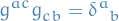
Raising and lowering of indices
Let be a vector space with .
A metric tensor on defines an isomorphism  by the map
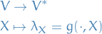
then

where  is the underlying field.
Therefore, we often write
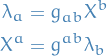
and we often surpress the difference between vector and covector , by simply writing  for the vector corresponding to
  , i.e.

which defines the raising and lowering operation often seen.
More generally, this works similarily for arbitrary tensors, e.g.  by the "lowering operation". Consider the example of a
  :
:

Signature of tensor
The signature of metric on is the number of negative values and the number of positive values  , and
, and  .
.
If  , i.e.
  for some
  , then the metric is positive-definite and thus defines an inner product!
The signature of a tensor is basis independent.
Lorentzian metrics
 are known as Lorentzian metrics, i.e. have one negative component.
First I wrote  , but this is not true! One can also have coefficients which are zero. So we don't necessarily have to have non-zero elements.
Let  and be a Lorentzian metric. Then we say is
- timelike if

- spacelike if

- null if

Null vectors form a "double cone" in the sense that if is null, then so is  for all
  .
.
In relativity, this is called the light-cone.
Future-directed vectors lie inside the future light-cone, and past-directed vectors lie inside the past light-cone.
Let  be a Riemannian manifold.
If there exists a nowhere vanishing vector field  , then admits a Lorentzian metric given by
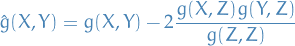
Let 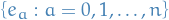 such that
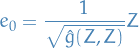
so that  has unit norm. From definition of , we have
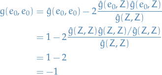
And
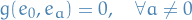
and

Therefore, in an orthonormal basis clearly has Lorentzian signature!
Psuedo-Riemannian manifolds
A metric tensor on a smooth manifold is a (0, 2)-tensor field which is symmetric and non-degenerate at every point  .
.
The pair is called a psuedo-Riemannian manifold.
So, for a psuedo-Riemannian manifold , the metric tensor has a particular signature at each point. Now, since the signature is integer-valued, by continuity, it must be constant from point to point. There are two types of signature which are of particular importance:
- : is positive-definite, then is a Riemannian manifold
 : is Lorentzian, then is a Lorentzian manifold
Let be a psuedo-Riemannian manifold. If is Lorentzian, i.e. has signature , then we say is a Lorentzian manifold.
In a coordinate basis, a metric tensor takes the form
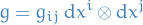
It is conventional to denote the symmetric tensor product of covectors by
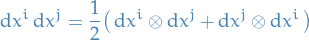
so we can write
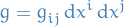
Examples
Consider
with Cartesian coordinates . The Euclidean metric is
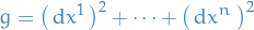
and
 is the Euclidean space.
Consider
with coordinates  . The Minkowski metric is

and
 is the Minkowski spacetime.
Consider
. In polar coordinates  the uni round sphere is
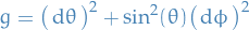
This is positive definite for all
 ; this corresponds to everywhere this chart is defined. However, the chart does not cover , so this does not fully define on . To fully define on , we need to consider an atlas on and ensure that is a smooth tensor field.
Length on Riemannian manifolds
Let
- be a Riemannian manifold.
 be a smooth curve.
The length of the curve is
![\begin{equation*}
L[\gamma] = \int_{a}^{b} \sqrt{g \big( \dot{\gamma}, \dot{\gamma} \big) \big|_{\gamma(t)}} \dd{t}
\end{equation*}](../../assets/latex/geometry_64be5ef79bddfc08fd821ddc3eac44b3e206aa3d.png)
where  is the tangent vector to the curve.
It may be checked that this definition is invariant under reparametrization of  . You can see this by noting that
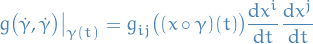
Because of this, the metric is often written as the "line element"
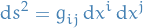
Consider defining a metric on by defining
![\begin{equation*}
d(p, q) = \inf_{\gamma} L[\gamma]
\end{equation*}](../../assets/latex/geometry_a581f2552e207f09552c436f9d3d410a4b20fa00.png)
i.e. the distance between two points  is defined to be the shortest path between the two points (wrt. length on the Riemannian manifold defined by ).
Clearly is non-negative, and vanish if and only if , since the term inside the integrand is positive for all values. It's also symmetric by the symmetry of the term inside the integrand.
Finally, one can show that the topology induced by is indeed the same as the topology defined on the manifold !
Let's define the open ball of radius  centered at as
![\begin{equation*}
B_r(p) = \left\{ q \in M : d(p, q) = \inf_{\gamma} L[\gamma] < r \right\}
\end{equation*}](../../assets/latex/geometry_08c0429031daf0fb6c6d1dd03d449146a9923690.png)
Observe then that if  for some chart
  , then the shortest line is simply the straight line in the Euclidean plane, i.e. directly corresponds with the open ball notion in the standard topology in . Therefore we only need to consider the case where
  is not fully contained in a single chart, but instead requires, say, two charts
  and
and  .
.
But, we know that the value takes on is basis-independent, and so we know the value will be exactly the same irregardless of the chart. Therefore it follows for multiple charts imediately as a consequence of the case where is fully contained in a single chart.
Or, we consider the determinant of the Jacobian when moving from  to
to  , and the explicitly write out the corresponding integral.
Defining a notion of length is not so straight-forward for Lorentzian manifolds.
A smooth curve is said to be timelike, spacelike, or null if the tangent vector  is the corresponding term for all !
Observe that most curves do not fit into this definition; the "type" of tangent vector can change along the curve, i.e. we can cross the boundaries of the "light-cones".
Thus, for a spacelike curve we have direct correspondance with the length defined on a Riemannian manifold, since  along . For the case of being timelike, we need a new notion.
Let
- be a Lorentzian manifold
- be a timelike curve with .
The proper time from along the curve is
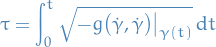
Again, this is invariant under reparametrization of .
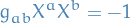
The tangent vector of a reparametrized curve  is given by

by the chain rule. Hence
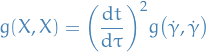
If is the proper time, then
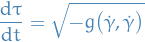
Hence
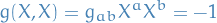
Grassman algebra and deRham cohomology
Notation
 , i.e. maps in s.t. composed with the projection from the total space to the base space of the tangent bundle form the identity. That is, maps a point in to it's fibre in , known as sections
- denotes a permutation in what follows section, NOT a projection as seen earlier
 denotes the set of permutations on letters / digits
 is the tensor product
![$(\circ)_{\textcolor{red}{[}m_1, \dots, m_n \textcolor{red}{]}} := \frac{1}{n!} \sum_{\pi \in \text{Perm}(n)} \text{sgn}(\pi) (\circ)_{\pi(m_1), \dots, \pi(m_n)}$](../../assets/latex/geometry_b3229ef146d9df851acbfc1c3ae8e70cb0b29c7e.png) is called the anti-symmetric bracket notation, where
is called the anti-symmetric bracket notation, where  denotes some "indexable object"
 is the same as anti-symmetric bracket notation, but dropping the
  , we call symmetric bracket notation
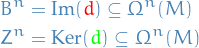
where
 is the exact forms and
  is the closed forms, where
  denotes the previous and
  the next
Grassman Algebra
The set of all n-forms is denoted

which naturally is a module since:
- sum of two n-forms is a n-form
- multiple of some
 is again in
We have a problem though: taking the tensor product of forms does not yield a form!
I.e. the space is not closed.
In what follows we're slowly building up towards a way of defining a product in such a way that we do indeed have the space of forms being closed under some additional operation (other than  and ), which is called the Grassman algebra.
We define the wedge product as follows:

defined by

e.g.

where the tensor product is just defined as

as usual.
Further, this allows us to construct the pull-back for some arbitrary form:
Let  and
and  be a smooth mapping between the manifolds.
This induces the pull-back:
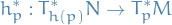
can be used to define
where  , which is the pull-back of the entire space rather than at a specific point .
Then,

where  is the push forward of a vector field.
The pull-back distributes over the wedge product:

The module defined

(where we've seen  and
and  before!)
Then  defines the Grassman algebra / exterior algebra of , with the being a bilinear map

is defined by linear contiuation of (wedge product for forms), which means that for example if we haven

where and  , and another
  , then

Now, as it turns out, we cannot define a differentiable structure on tensors on some manifold . But do not despair! We can in fact do this on anti-symmetric tensors, i.e. forms, we can indeed define a differentiable structure without any further restrictions on the manifold!
The exterior derivative operator

where
![\begin{equation*}
\begin{split}
\big( d \omega \big) \big( X_1, \dots, X_{n + 1} \big) := &\sum_{i=1}^{n + 1} (-1)^{i + 1} X_i \Big( \omega \big( X_1, \dots, \cancel{X_i}, \dots, X_{n + 1} \big) \Big) \\
&+ \sum_{i < j} (-1)^{i + j} \omega \big( [X_i, X_j], X_1, \dots, \cancel{X_i}, \dots \cancel{X_j}, \dots X_{n + 1} \big)
\end{split}
\end{equation*}](../../assets/latex/geometry_0197dfb7477c73d7e52174d86b4ff15bf6f70088.png)
i.e. since takes entries we leave out the i-th entry, and ![$[X_i, X_j]$](../../assets/latex/geometry_523877f4ed3c5ddf96c2e5035f0e6d46e5ab27ba.png) is the commutator.
is the commutator.
Equivalently, this can also be defined as
where we hare using multi-indexing, and
with , and so
Commutator of two vector fields  is given by
![\begin{equation*}
[X, Y]f := X \big( Yf \big) - Y \big( Xf \big)
\end{equation*}](../../assets/latex/geometry_ce468b280d9bb587cd8c9d0860ca4345a73a6239.png)
for  .
.
A geometrical interpretation of  ..
..
Let be the endpoint of concatenating  with
with  , and
, and  be the endpoint of starting with and concatenating with . Then one can show that
where is the i-th component of some chart. Here we have Taylor expanded in which case the first-order terms turn out to cancel, and we get the above.
Let and  .
.

If we have the smooth map , then
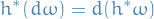
where we observe that the are "different":
- LHS:

- RHS:

which is why we use the word "commute" rather than that they are "the same" (cuz they ain't)
Further, action of extends by linear continuation to  :
:

where denotes the Grassman algebra.
Exterior power
Let be a vector space with  .
.
Then the exterior power is defined as  , a subspace of the Grassman algebra,

In the case where  , we have
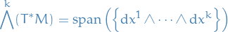
Then we have
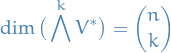
Physical examples
Maxwell electrodynamics
Let be the field strength, i.e. the Lorentz force:
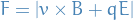
then is a two-form (since it maps both and to ), and we require

which is called the homogenous Maxwell equations.
Since is a two-form on the reals, we know from Poincaré lemma that if a n-form is closed on and thus we must exact, thus

for some  . is called the gauge potential.
de Rham Cohomology
The following theorem has already been stated before, but I'll restate it due to it's importance in this section:

where is the exterior derivative.

and
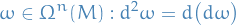
in local coords:
![\begin{equation*}
\begin{split}
dw &= \big( \partial_b \omega_{a_1, \dots, a_n} \big) dx^b \wedge dx^{a_1} \wedge \dots \wedge dx^{a_n} \\
&= \big( \partial_{\textcolor{red}{[} b} \omega_{a_1, \dots, a_n \textcolor{red}{]}} \big) dx^b \wedge dx^{a_1} \wedge \dots \wedge dx^{a_n}
\end{split}
\end{equation*}](../../assets/latex/geometry_194f30bdc4253d595f0a988762cc3ebb15ed6c6a.png)
(remember we're using Einstein summation), where we've used the fact that ![$A_{ab} B^{\textcolor{red}{[}a, b \textcolor{red}{]}} = A_{\textcolor{red}{[}a, b \textcolor{red}{]}} B^{ab}$](../../assets/latex/geometry_3f8af7fde955b2be7c685ad733a5e079d4e618ff.png) , which gives us
, which gives us
![\begin{equation*}
\begin{split}
d \big( d \omega \big) &= \big( \partial_{\textcolor{red}{[} c} \partial_b \omega_{a_1, \dots, a_n \textcolor{red}{]}} \Big) dx^c \wedge dx^b \wedge dx^{a_1} \wedge \dots dx^{a_n} \\
&= 0
\end{split}
\end{equation*}](../../assets/latex/geometry_27af035f1636181d44cf936d1b3ab45b43153ea6.png)
where the last equality is due to Schwartz (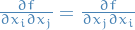 under certain conditions).
implies that there exists a sequence of maps such that

We then observe that:
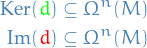
where the above theorem tells us that:

Now, we introduce some terminology:

We then say that is called:
- exact if

- closed if

which is equivalent to the exact and closed definitions that we've seen before, since  for some
  is exact, i.e. . Observe that we here consider as a mapping
  rather than
  , thus the different colored mappings are sort of the same but sort of not :)
As we know from Poincaré lemma, there are cases where

but then you might wonder, if it's not the case: how would one quantify the difference between and ?
The n-th deRham cohomology group is the quotient vector space
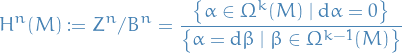
where on we have equivalence relation:

and we write (this is just notation)

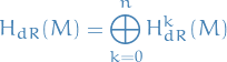
defines the deRham cohomology.
This we can equip with a "wedge"
![\begin{equation*}
\begin{split}
\wedge: \quad & H_{dR}^k(M) \times H_{dR}^l(M) \overset{\wedge}{\longrightarrow} H_{dR}^{k + l}(M) \\
& (\alpha, \beta) \mapsto [\alpha] \wedge [\beta] := [\alpha \wedge \beta]
\end{split}
\end{equation*}](../../assets/latex/geometry_d22017b5866b16526c21e3bcc65d0c019a6bcc69.png)
which we can check is well-defined.
The idea of de Rham cohomology is to classify the different types of closed forms on a manifold.
One performs this classification by saying that two closed forms  are cohomologous if they differ by an exact form, i.e.
  is a exact:

or equivalently,

where  is the set of exact forms.
Thus, the definition of n-th de Rham cohomology group is the set of equivalence classes with the equiv. relation described above; that is, the set of closed forms in  modulo the exact forms.
Further, framing it slightly different, it might become a bit more apparent what we're saying here.
Observe that

Since 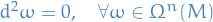 , then clearly

And further, it turns out that by partitioning all the closed forms by taking the "modulo" the exact forms, we get a set of unique and disjoint partitions (due to this being an equiv. relation).
That is,

This is quite a remarkable result, since all our "previous" work depends on the exterior derivative of the local structure, and then it turns out that  only depends no the actual topology of the manifold! Woah dude!
We have the following example:

Since 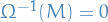 then
then  , therefore
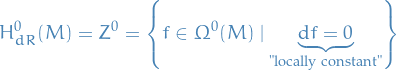
If is connected, then

with the bijection ![$[f] \mapsto f(a)$](../../assets/latex/geometry_8f860ec87ffad0cc122ae8173404df0eb4b0d3ec.png) for some (which is arbitrary since is connected).
for some (which is arbitrary since is connected).
Assume ![$c: [0, 1] \to M$](../../assets/latex/geometry_c76b9f4aaa06da2bda01679891f49d6c15696c15.png) is smooth, then FTC implies
is smooth, then FTC implies
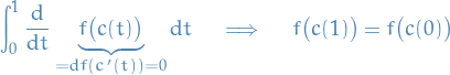
Let  be . then it induces
![\begin{equation*}
\begin{split}
F^*: \quad & H_{dR}(M) \to H_{dR}(N) \\
& [\alpha] \mapsto F^*[\alpha] := \big[ F^* \alpha \big]
\end{split}
\end{equation*}](../../assets/latex/geometry_427074b984042687fa1a7dffc6699f49c838ae5d.png)

and so
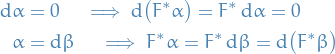
shows that it's well-defined.
And it is a homomorphism:
![\begin{equation*}
F^* \big( [\alpha] \wedge [\beta] \big) = F^* [\alpha \wedge \beta] = [F(\alpha \wedge \beta) ] = [F^* \alpha \wedge F^* \beta] = [F^* \alpha] \wedge [F^* \beta] = F^*[\alpha] \wedge F^*[\beta]
\end{equation*}](../../assets/latex/geometry_34c99199d9224ca73202be20f357e06a0949fe24.png)
Let
![\begin{equation*}
\begin{split}
F: \quad & N \times [0, 1] \to M \\
& (a, t) \mapsto F_t(a) := F(a, t)
\end{split}
\end{equation*}](../../assets/latex/geometry_dff211fd6ba546e35da4fb86ff9dc17b7c97e8f1.png)
be "smooth" in the sense that is smooth on  for any
  .
Then
.
Then
![$[\alpha] \in H_{dR}^k(M)$](../../assets/latex/geometry_ec1da94fd83042cf9b2065e5795b8b042fdf3644.png) then
then ![$F^* \alpha \in \Omega^K \big( N \times [0, 1] \big)$](../../assets/latex/geometry_50455de99aecee5c062d9c3bb9059d7e1d17a06d.png) , and let
, and let
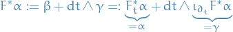
so  and
and  .
Then
.
Then

which implies
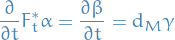
Integrating

![\begin{equation*}
\therefore \quad \big[ F_1^* \alpha \big] = \big[ F_0^* \alpha \big], \quad \forall \alpha
\end{equation*}](../../assets/latex/geometry_d2cb73fab93c826e042cb7bf768f1f2e7032f58c.png)
hence

From this we can restate Poincaré Lemma using the deRham cohomology.
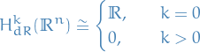
![\begin{equation*}
\begin{split}
F: \quad & \mathbb{R}^n \times [0, 1] \to \mathbb{R}^n \\
& (x, t) \mapsto tx
\end{split}
\end{equation*}](../../assets/latex/geometry_dcfb3e49e0b681bf75542cd9de9f33292c08f9ed.png)
Then
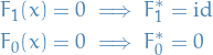
for  .
.
So ![$[\alpha] \in H_{dR}^{k > 0}(\mathbb{R}^n)$](../../assets/latex/geometry_a155bff37224c8d568d47010698762e210ee7e6a.png) , therefore
, therefore
![\begin{equation*}
[\alpha] = F_1^* [\alpha] = F_0^*[\alpha] = 0 \quad \implies \quad H_{dR}^{k > 0}(\mathbb{R}^n) = 0
\end{equation*}](../../assets/latex/geometry_ef5c6f28e5c9a0d05a2e8c6039f5086236bf436e.png)
Summary
- From we get the sequence with inclusions where always the images are included in the kernels of the next map.n
- Then if we want to quantify how much the images diviate from the kernel, we can quantify by "modding out" the closed forms, , from the exact forms, .
- We then learn purely topological invariants,

So now we want to show that this is
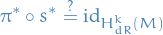

First we show that
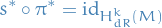
and then we need to show that also

We have
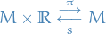
with

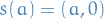


Therefore,
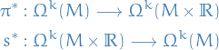
Then we have
![\begin{equation*}
\pi \circ s = \id_M \quad \implies \quad s^* \circ \pi^* = \id_{\Omega^k(M)} \quad \implies s^* \pi^* [\alpha] = \big[ s^* \pi^* \alpha \big] = [\alpha]
\end{equation*}](../../assets/latex/geometry_68cc59f91903cbd8436a394151b0aa83535f7adc.png)
which implies
Now we show
It's sufficient to show that on  ,
, 

(such a is called a chain homotopy)
If we have such a , then
![\begin{equation*}
\begin{split}
\pi^* \circ s^* [\alpha] &= \big[ \pi^* s^* \alpha \big] \\
&= \big[ \alpha \pm (K \dd{} + \dd{K}) \alpha \big] \\
&= \big[ \alpha \pm K \underbrace{\dd{\alpha}}_{= 0} \pm \underbrace{\dd{K \alpha}}_{\text{exact}} \big] \\
&= [\alpha]
\end{split}
\end{equation*}](../../assets/latex/geometry_145dea253b0c702d098713f4347fd3acd73de0a3.png)
Construction of : "integration along the fibre"

Let

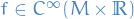

In we have two kinds of forms:
So we define to
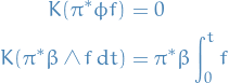
where
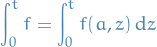
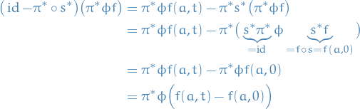
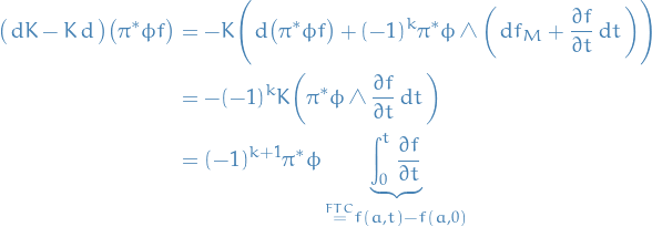
where on the LHS initially  vanish, since
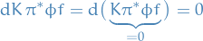
Upshot:

which is an identity for "forms of the form"  ; now we need for
  also.
also.
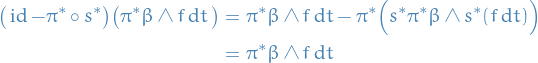
where we have used the fact that
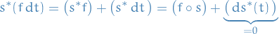
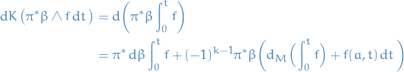
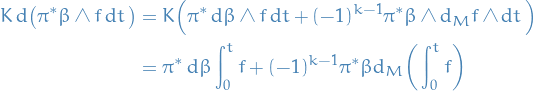
Comparing terms in  and
and  , we see

Upshot:

Thus we have such a  , and hence
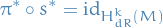
which concludes our proof.
Lie Theory
Notation
 often used as short-hand notation for the K-vectorspace
  when this vector space is further equipped with the Lie brackets
 ![$[\![ \cdot, \cdot ]\!]$](../../assets/latex/geometry_d6b3dbf677410cdec3ec3460fb6fa51409925708.png) , i.e. when writing
, i.e. when writing
![\begin{equation*}
(L, [\![ \cdot, \cdot ]\!])
\end{equation*}](../../assets/latex/geometry_6f28788660d722322bed435dd221b9bc0330e915.png) refers the underlying K-vectorspace.
refers the underlying K-vectorspace.
 is the set of left-invariant vector fields in the Lie group
  refers to two vector spaces being isomorphic (which is not the same as, say, a group isomorphism)
- denotes the abstract Lie-brackets, i.e. any function which takes two arguments as satisfy the properties of a Lie bracket.
 denotes the particular instance of a Lie bracket defined by

known as the commutation relation
 refers to the 0th fundmantal group / path components
 refers to the 1st fundamental group
 denotes the connected component of the identity
- Submanifold refers to embedded submanifold
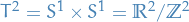 denotes the 2-torus
 denotes the space of vector fields
 denotes that acts on as a group
 denotes the Lie algebra generated by the Lie group
 - denotes a Lie group, and
 denotes the corresponding Lie algebra
  and
and  denotes the space of morphisms of Lie group and Lie algebra reps
- Sometimes you might see
 or something for vector fields
  (though I try to avoid it) which really means
  and similarily
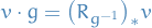
Stuff
A Lie group  is
is
a group with group operation
:

where
 denotes that the group could be commutative, but is not necessarily so.
- is a smooth manifold and the maps:
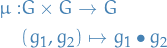
where
 inherits smooth atlas from , thus is a map between smooth manifolds.

are both smooth maps.
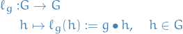
Each left translation of a Lie group  is an isomorphism but NOT a group isomorphism.
It is also a diffeomorphism on , by the definition of a Lie group.
Let  and
and  be Lie groups
If  is a smooth / analytic map preserving group structure, i.e.

then is a morphism of Lie groups.
- Lie groups do not have to be connected, neither simply-connected
- Discrete groups are Lie groups
Let
- be a Lie group
- be the connected component (which always exists around identity) of

- Then is a normal subgroup in and
 is a Lie group itself.
  is a discrete group
First we show that
is indeed a Lie group. By definition of a Lie group, the inversion map
is continuous. The image of a connected topological space under a continous map is connected, hence
takes  to a connected comp of containing the identity, since
Similar argument for
 . Hence is a Lie group.
At the same time, conjugation
. Hence is a Lie group.
At the same time, conjugation

is cont. in
 for all
  . Thus
  is a conn. comp. of which contains
  since
since  .
.

Let
 be the quotient map. is an open map (i.e. maps open to open) since
  is equipped with the quotient topology. This implies that for every we have
i.e. it's open. This implies that every element of
is an open subset, hence the union of all elements in cover and each of them open, i.e. we have an open covering in which every open subset contains exactly one element of (which is the definition of a discrete topological group).
 is the (trivial) projection map
Show that
 is a Lie group.
Let be a connected manifolds, ,
is a Lie group.
Let be a connected manifolds, ,  , and
, and

be cont.
 be universal covers,
  and
and  with
with
Then
lifts to  s.t.
s.t.

Choose
 s.t.
s.t.  implies that
  lifts in a unique way to
  taking
  .
Same trick works for
.
Same trick works for  .
.
 is discrete and central
Lie subgroups
A closed Lie subgroup of a Lie group is a (embedded) submanifold which is also a subgroup.
A Lie subgroup of a Lie group is an immersed (as opposed to embedded) submanifold which is also a subgroup.
- Any closed Lie subgroup is closed (as a submanifold)
- Any subgroup of a Lie group which is a closed subset is a closed Lie group.
- connected Lie group, neighborhood of
 , then generates .
 - is a morphism of Lie groups, and is connected.
If
 is surjective, then is surjective.
- subgroup generated by , then is open in because
 , we have
  is open neighborhood of in . Then
- Open subset of a manifold is a submanifold is a submanifold
- is closed Lie subgroup
- is closed
- is closed and open
- is connected component in
-
 , since is connected
- Open subset of a manifold is a submanifold
- Inverse function theorem says that
 is surjective onto some neighborhood
  , Since an image of a group morphism is a subgroup, and generates , is surjective.
Example
 and
and  with
with
Then it is well-known (apparently) that the image of this map is everywhere dense in  , and is often called the irrational or dense winding of , and the map is open "one way" but the "other way".
This is an example of a Lie subgroup which is NOT a closed Lie subgroup. The image of the map  is a Lie subgroup which is not closed. It can be shown that if a Lie subgroup is closed in , then it is automatically a closed Lie subgroup. We do not get a proof of that though, apparently.
Factor groups
- As in for discrete groups, given a closed Lie subgroup
 , we can define notion of cosets and define
  as the set of equivalence classes.
 - Following theorem shows that the coset space is actually a manifold
Let
- Lie group
- closed Lie group


Then is a submanifold of  and there exists a fibre bundle with
  , where
  is the canonical map, with as it's fibre.
The tangent space is given by
is the canonical map, with as it's fibre.
The tangent space is given by
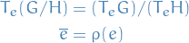
Further, if is a normal closed Lie subgroup then has a canonical structure of a Lie group (i.e. transition maps are smooth and the smooth structure does not depend on the choice of and (see proof).
Let
 be the canonical map
- and
Then  is a (embedded) submanifold in as it's an image of under diffeomorphism
  .
Choose a submanifold
.
Choose a submanifold  such that
  and is traversal to the manifold , i.e.
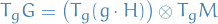
which implies that  .
.
Let  be a sufficently small neighborhood of in . Then the set

is open in . This follows from the IFT applied to the map  .
.
Consider  . Since
  is open,
  is an open neighborhood of
  in and the map
  is a homeomorphism.
This gives a local chart for by
is a homeomorphism.
This gives a local chart for by  , where denotes a chart map for . At the same time this shows that
  is a fibre bundle with fibre .
GET CONFIRMATION ABOUT THIS.
With the the atlas  we see that the transition maps are smooth by the smoothness of and
  . Further, observe that choosing any other and does not alter the proof, since still holds, and therefore ???
The above argument also shows that the push-forward of , i.e.  has the kernel

In particular,  gives the isomorphism (since
  is an isomorphism)

as wanted.
REMINDER:
If is a fibre bundle with fibre , then there exists a long exact sequence of homotopy groups

Exact means that  with
with  .
.
Let be a closed Lie subgroup of a Lie group .
- connected
 where
where  . In paricular, if and are both connected, then so is .
 - connected, connected

Push-forward on fields
- Recall that we we're able to generalize the pull-back from covectors to covector fields.
- Unfortunately not quite the same when we try to generalize the push-forward on a vector to vector fields
- It turns out, if the underlying smooth map is a diffeomorphism, then we can in fact extend the push-forward to vector fields!
What does this mean? It means that on a Lie group we can in fact construct a diffeomorphism using the left translations, and thus a push-forward from to , i.e. we can map vector fields to vector fields in the group !
We can push forward on vector field on to another vector field, defined
where  ,
,  .
.
Let be a Lie group, and a vector field on , then is called left invariant vector field, if for any

Alternatively, one can write this as
where we write the map pointwise on the vector field.
Alternatively, again,  and
and 
 &= \big[ \big( Xf \big) \circ \ell_g \big] (h) \\
X \big( f \circ \ell_g \big) &= \big( Xf \big) \circ \ell_g
\end{split}
\end{equation*}](../../assets/latex/geometry_4c739c29ec8af1a4e221f0692bca2acf1e9ceaed.png)
Similarily we can define right invariant and bi-invariant (both left- and right-invariant).
The set of left-invariant vector fields of a Lie group can be denoted

where  is a
is a  module.
We observe that the following is true:
which implies that is a module.
Example: acting on space of vector fields
yields acts on
Then push-forward

If and 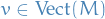 , we let
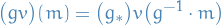
If 
 then acts on
  .
.
Example: acting on dual space of
Let  be a dual space to , i.e. cotangent space.
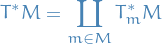
is again a vector bundle called the cotangent bundle.
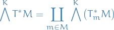
is a vector bundle as well and it sections called k-forms.
yields that  is a
is a  .
.
Lie Algebra
A one-parameter subgroup corresponds to an map
 is a morphism of Lie groups


 s.t. integral curve
  with initial condition
  exists and is unique.
Moreover, the map (called the flow)
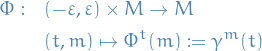
is smooth.
 there exists a unique one-parameter subgroup corresponding to .
Choose  and let
  be the corresponding left-invariant vector field,
  be the time flow of . Then
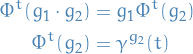
satsifies
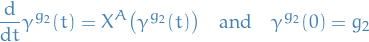
Furthermore,  satisfies
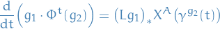
by the chain rule. Then 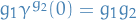 .
.
In other words, the RHS and LHS satisfy the same diff. eqn. but solutions are unique by thm:uniqueness-of-ODE-solution-and-flows.
For it to be a morphism, we observe that it preserves the group operation. Letting 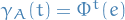 , we have
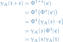
For  , let
, let  be a one-param. subgroup..
Identify  , then
 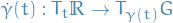 is a composition
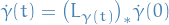
Therefore is an integral curve for a left-invariant vector field corresponding to  .
.
Hence, is unique.
An abstract Lie algebra ![$(L, +, \cdot, [\![ \cdot, \cdot ]\!])$](../../assets/latex/geometry_a56f433228bc871264668cbcbcd5ed4fe8b9fa01.png) is a K-vectorspace equipped with an abstract lie bracket that satisfies:
is a K-vectorspace equipped with an abstract lie bracket that satisfies:
- bilinear (in ):
![$[\![ \cdot, \cdot ]\!]: L \times L \to L$](../../assets/latex/geometry_d97b5213416e39e87a7e2905f02d51f63061ca50.png)
- anti-symmetric:
![$[\![ x, y ]\!] = - [\![ x, y ]\!]$](../../assets/latex/geometry_645b8fe40e1713d8bed1d4b225ea2b6f43f49f36.png)
Jacobi identity:
![\begin{equation*}
[\![ x, [\![ y, z ]\!] ]\!] + [\![ y, [\![ z, x ]\!] ]\!] + [\![ z, [\![ x, y ]\!] ]\!] = 0
\end{equation*}](../../assets/latex/geometry_808cd05222c93009dec20d6d739ff736a66698db.png)
One might wonder why we bother with these weird brackets, or Lie algebras at all; as we'll see, there is a correspondance between Lie groups, which are geometrical objects, and these Lie algebras, which are linear objects.

Equivalently, one could do the same as in Thm. thm:left-invariant-vector-fields-isomorphic-to-tangent-identity for right-invariant vector fields  , thus making
  .
.
Further, for the bi-invariant vector fields defined

we also have being isomorphic to the left- and right-invariant vector fields:

We start with the following corollary
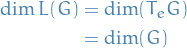
We need to construct a linear isomorphism
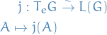
where

where  denotes at the point .
That is, we push forward the vector-field at the point  for every point , thus creating a vector at every point.
We now prove that it's left-invariant vector field:
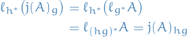
- It's clearly linear, since
 and the push-forward on a vector-field at the point ,
  , is by definition linear.
  is injective:

which can be seen from

- is surjective:
Let
 , i.e. is a left-invariant vector field. Then we let
  be some vector field associated with , defined by
Consider:
which implies

Hence, as claimed,

Which means that as a vector space we can work with  to prove properties of the vector-field of left-invariant vector field!
Only problem is that we do not have the same algebra, i.e.
and we would really like for the following to be the case
![\begin{equation*}
\Big( T_e G, [\![ \cdot, \cdot ]\!] \Big) \cong_\text{alg} \Big( L(G), \comm{\cdot}{\cdot} \Big)
\end{equation*}](../../assets/latex/geometry_22c3b323892241f5bc219a51b8eb24094dc7f3c6.png)
that is, we want some bilinear map ![$[\![ \cdot, \cdot ]\!]: T_e G \times T_e G \to T_e G$](../../assets/latex/geometry_b4115e543d1ec9228f45cda16effc00341a3414a.png) s.t.
s.t.
![\begin{equation*}
j \Big( \textcolor{red}{[\![ A, B ]\!]} \Big) = \comm{j(\textcolor{red}{A})}{j(\textcolor{red}{B})}
\end{equation*}](../../assets/latex/geometry_3ff6b4d8a3225c8bf848558ddc6bd5ab74295d62.png)
Thus, we simply define the commutation brackets on , such that
![\begin{equation*}
\underbrace{\textcolor{red}{[\![ A, B ]\!]}}_{\in T_e G} = \underbrace{j^{-1} \bigg( \comm{j(\textcolor{red}{A})}{j(\textcolor{red}{B})} \bigg)}_{\in L(G)}
\end{equation*}](../../assets/latex/geometry_8ca708871554e8e24cab3fa792f975edfd24f982.png)
as desired we get
Example of Lie Algebra
 is a
is a ![\begin{equation*}
\Big( \Gamma(TM), +, \cdot, [\![ \cdot, \cdot]\!] \Big)
\end{equation*}](../../assets/latex/geometry_6847f96d6e7aeb2e9995777bbd448fa2756c2be4.png)
Examples of Lie groups
Unit circle
where we let the group operation  , i.e. multiplication in
  .
.
Whenever we multiply a two complex numbers which are both unit length, then we still end up on the unit-circle.
General linear group

equipped with the  operation, i.e. composition. Due to the nature of linear maps, this group is clearly satisfies
  (but not
  ), hence it's a Lie group.
Why is GL a manifold?
 can be represented in
  (as matrices), and due to the
  the set is also open.
Thus we have an open set of on which we can represent as
Relativistic Spin Group
In the definition of the relativistic spin groups we make use of the very useful method for constructing a topology over some set by inheriting a topology from some other space.
- Define topology on the "components" of the larger set
- Take product topology
- Take induced subset-topology
Proof / derivation
To define the relativistic spin group  we start with the set
- As a group
We make
into a group  :
:
i.e. matrix multiplication, which we know is ANI (but not commutative):
- Associative
- Exists neutral element
- Invertible (since we recognize
 )
)
- As a topological space
From this group, we can create a topological space
 :
:
Define topology
 on by virtue of defining "open balls":

which is the same as we do for the standard topology in
.
Take the product topology:

Equip
 with the induced subset topology of the product topology over
  , i.e.

Verify that we have
, with  as given above, is a topological manifold. We do this by explicitly constructing the charts which together fully covers , i.e. defines an atlas of :
First chart
:
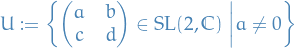
and the map
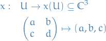
which is continuous and invertible, with the inverse:
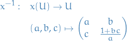
hence
 is a homeomorphism, and thus is a coordinate chart of .
Second chart
 :
:
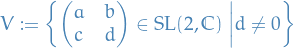
and the map
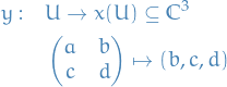
which is continuous and invertible, with the inverse:
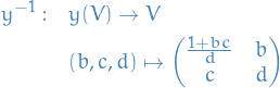
Third chart
 :
:
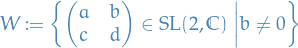
and the map
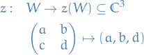
which is continuous and invertible, with the inverse:
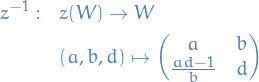
Then we have an atlast in
 , since these cover all of , since the only case we're missing is when all
  , which does not have determinant
  , therefore is not in .
Hence, is a complex topological manifold, with
, therefore is not in .
Hence, is a complex topological manifold, with
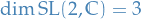
- As a differentiable manifold
Now we need to check if
 is differentiable manifold (specifically, a
  ); that is, we need the transition maps to be "
 compatible", where ? specifies the order of differentiability.
One can show that the atlast
 defined above is differentiable to arbitrary degree. We therefore let be the maximal atlast with differentiability to arbitrary degree, containing the atlast we constructed above. This is just to ensure that in the case we late realize we need some other chart with these properties, then we don't have to redefine our atlas to also contain this new chart. By using the maximum atlas, we're implicitly including all these possible charts, which is convenient.
One can show that
above defines open subsets, by observing that the subset where  is closed, hence the complement () is open.
- As a Lie group
As seen above, we have the group
 , where is a manifold to arbitrary degree, with the maximum atlas containing
  as defined previously.
To prove that this is indeed a Lie group, we need to show that both the following maps:
and
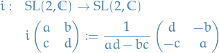
are both smooth.
Differentiability is a rather strong notion in the complex case, and so one needs to be careful in checking this. Nonetheless, we can check this to the arbitrary degree.
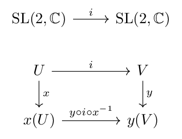
We observe that the Fig. fig:commutation-diagram-inverse-relativistic-spin-group-charts is the case, since the inverse map restricted to
, where , is then mapped to  , i.e. the image is .
We cannot talk about differentiablility on the manifold itself, hence we say
is differentiable if and only if the map  is differentiable (since we already know and are differentiable). We observe that

which is most certainly a differentiable map. We've used the fact that all these matrices have
 in the inverse above.
Performing the same verification for the other charts, we find the same behavior. Hence, we say that
, on the manifold-level, is differentiable.
For
we can simply let the product-space  inherit the smooth atlast on , hence is also smooth.
That is, the composition map
and the inverse map are both smooth for the group , hence is a complex 3-dimensional Lie group!
- TODO As a Lie algebra
In this section our aim is to construct the Lie algebra
 of the Lie group .
We will use the standard notation of
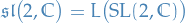
Recall
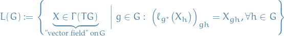
i.e. it's the set of left-invariant vector fields.
Further, recall
where
Now, we need to equip
with the Lie brackets:
![\begin{equation*}
\begin{split}
[\![ \cdot, \cdot ]\!]: \quad & T_{\mathrm{id}} \ \mathrm{SL}(2, \mathbb{C}) \times T_{\mathrm{id}} \ \mathrm{SL}(2, \mathbb{C}) \to T_{\mathrm{id}} \ \mathrm{SL}(2, \mathbb{C}) \\
& (A, B) \mapsto [\![ A, B ]\!] := \ell_{(g^{-1})^*} \comm{\ell_{g^*} A}{\ell_{g^*} B}
\end{split}
\end{equation*}](../../assets/latex/geometry_e53a4748e81afcc8e83456172a4e5b207ce9be51.png)
where
To explicitly write out this
, we use the chart since  . For any
  , we have

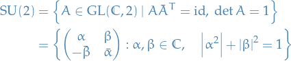

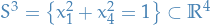 .
.
Classification of Lie Algebras
Notation
- In this section we mainly consider complex Lie algebras
- Commutation between two Lie algebras is denoted

 is the direct sum between Lie algebras
 is the semi-direct sum between Lie algebras
 refers to the span of the set of vectors using coefficients from field
  defined
  is the killing form
The roots of a roots of a Lie algebra with Cartau subalgebra
is denoted

- Set of fundamental roots of Lie algebra

Similar stuff
If a representation is reducible, then it has a non-trivial subrepresentation  and thus, can be included in a short exact sequence

where  is the inclusion mapping, and
  is the canonical mapping.
Apparently, the natural question is whether the above sequence splits, i.e. whether
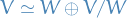
If so, one can iterate the process to decompose into a direct sums of irreducibles.
Example of non-semisimple representation
Let  and so
  .
.
Note: I find the below confusing. I think a better approach is to note that is commutative and so the rep must also be commutative. The only matrices which are commutative are the diagonal matrices, hence we have full reducibility.
The a representation of  is the same as a vector space with a linear map
  . Every such map is of the form

for some arbitrary  .
.
The corresponding representation of the group is given by

Thus, classiying representations of is equivalent to classifying linear maps  up to a change of basis.
Such a classification is known (it's the Jordan normal form!), but is non-trivial.
Now consider the case where is an eigenvector of , then the one-dimensional space  is invariant under , and thus is a subrerepresentation in . Since every linear operator in a complex vector space has an eigenvector, this shows that every representation of is reducible, unless it is one-dimensional. We just saw above that the one-dimensional rep is indeed irreducible, hence the only irreducible representations of are one-dimensional.
One can see that writing a representation given by
as a direct sum of irreducible representations is equivalent to diagonalizing ; recall that the direct sum of two vector subspaces and is the sum of the subspaces in which and only have  in common, and the direct sum of matrices is
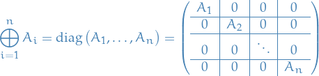
Therefore, a representation is completely reducible if and only if is diagonalizable. Since not every linear operator is diagonalizable, not every representation is completely reducible.
More stuff
Let  be a representation of (respectively ) and
  be a diagonalizable intertwining operator.
Then each 
 is a subrepresentation (of Lie group), so

In particular, for any  (the center of ) such that
  is diagonalizable, decomposes into a direct sum of
  .
.
Stuff
Every finite-dim. complex Lie algebra  can be decomposed as

where:
- is a Lie sub-algebra of which is solvable , i.e.:
![\begin{equation*}
\{ \comm{r_1}{r_2} \mid r_1, r_2 \in R \} = \comm{R}{R} \supseteq \comm{\comm{R}{R}}{\comm{R}{R}} \supseteq [ \ \cdot \ , \ \cdot \ ] \supset \dots \overset{!}{=} \{ 0 \}
\end{equation*}](../../assets/latex/geometry_6671184e98683264e0442ec78129efa3515d3c9b.png)
 are simple Lie algeabras, i.e.
 is non-abelian
 contains no non-trivial ideals, where:
- An ideal means some sub-vector space
 s.t.
s.t.  , i.e. if you bracket the sub vector spaces from the outside, then you're still in the ideal .
  is clearly ideal since
- An ideal means some sub-vector space
The direct sum
between Lie algebras is defined as:
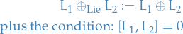
semi-direct sum

Which saying that we can always decompose a complex Lie algeabra in a solvable , semi-direct sum, and a direct sum between simple Lie algebras.
Every Lie algebra can be decomposed into a semi-direct sum between a solvable Lie algebra and a direct sum between simple Lie algebras
An example of solvable Lie algebra is the upper-triangular matrices.
An example of un-solvable Lie algebra is  since taking the commutator gives you the space itself, i.e.

A Lie algebra that has no solvable part, i.e.  is called semi-simple.
A Lie algebra is called simple if there are no ideals other than  and itself, and it is not abelian.
If is simple, then no solvable ideals other than (possibly) . Therefore

since otherwise we would not be able to repeatedly apply commutators and eventually reach . This is a contradiction, concluding our proof.
We say the radical of is the maximal sovlable ideal which contains every other solvable ideal.
We denote the radical of a  .
.
A representation is called semi-simple or completely reducible if it is isomorphic to a direct sum of irreducible representations, i.e.

In this case, it is common to group isomorphic direct summands, and write
the number  is called the multiplicity of the subrepresentation
  .
.
It turns out it's quite hard to classify the solvable Lie algebras , and simpler to classify the semi-simple Lie algeabras. Thus we put our focus towards classifying the semi-simple Lie algebras and then using these as building blocks to classify the full Lie algebra of interest.
 is a complex
  , then define
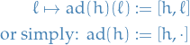
The bililinear map
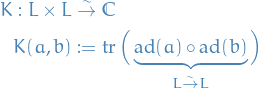
is called the killing "form" (it's a symmetric map, so not the kind of form you're used to).
And we make the following remarks about the Killing form:
- is finite-dim. thus the
 is cyclic, hence
- is solvable if and only if
![\begin{equation*}
K \big( [L, L], L \big) = 0
\end{equation*}](../../assets/latex/geometry_b07f4ae3c7a724187f9bafe3786cdaf86d28ffa0.png)
- semi-simple (i.e. no solvable part) if and only if is non-degenerate:

- invariant since
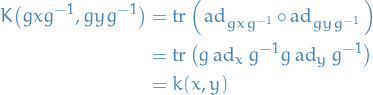
Now, how would we then compute these simple forms?
Now consider, for actual calculations, components of  and wrt. a basis:
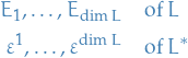
Then
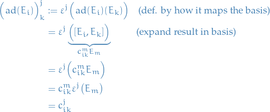
where  are just coefficients of expanding the commutation in the space of the complex numbers, which we clearly can do since
  . These coefficients are called the structure constants of wrt. chosen basis.
The killing form in components is:
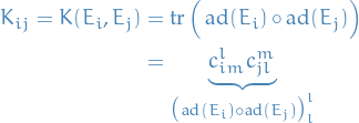
Where the last bit is taking the . Thus, each component of the killing form is given by

We then empasize that is semi-simple if and only if is a psuedo-inner product (i.e. inner product but instead of being positive-definite, we only require it to be non-degenerate).
One can check that is anti-symmetric wrt. killing form a (for a simple Lie algeabra, which implies semi-simple).
A Cartau subalgebra of a Lie algebra ![$(L, [\cdot, \cdot])$](../../assets/latex/geometry_634f6124e0db94362d3f15d111b0c39a7a77e48f.png) is:
is:
 as a vector subspace
maximal subalgeabra of
and that there exists a basis:

of
that can be extended to a basis of

such that the extension vectors
 are eigenvectors for any where
  :
:
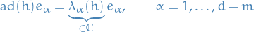
where the eigenvalue
 depends on since with any other we have a different map
Now, one might wonder, does such a Cartau subalgebra exists?!
- Any finite-dimensional Lie algebra posses a Cartau subalgebra
- If is simple Lie algebra then is abelian, i.e.
![$[H, H] = 0$](../../assets/latex/geometry_5f73d831d874e1a9538e1a152736b3161b14bd83.png)

is linear in . Thus,

I.e. we can either view  as a linear map, OR as a specific value
  . This is simply equivalent of saying that

The  are the roots of the Lie algebra, and we call
the root set.

A set of fundamental roots such that
 linearly independent,
Then
 such that
Observe that the makes it so that we're basically choosing either to take all the positive or all the negative , since they are linearly independent, AND this is different from saying that  !!! Since we could then have some negative and some positive. We still need to be able to produce
  from , therefore we need the .
And as it turns out, such a can always be found!
The fundamental roots of span the Cartau subalgebra

buuut note that is not unique (which is apparent by the fact that we can choose  for the expressing the roots, see definition of fundamental roots).
If we let  , then we have
We define the dual of the Killing form as  defined by
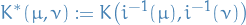
where we define
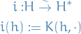
where  exists if is a semi-simple Lie algebra (and thus of course if it's a simple Lie algebra).
If we restrict the dual of the Killing form  to
to  (as opposed to
  ), that is,

and

with equality if and only if  .
.
Then, on  we can calculate lengths and angles.
In particular, one can calculate lengths and angles of the fundamental roots of (all roots are spanned by fundamental roots => can calculate such on all roots).
Now, we wonder, can we recover precisely the set from the set ?
For any  define
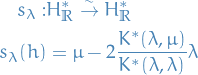
which is:
- linear in
- non-linear in
and such  is called a Weyl transformation, and
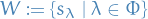
called Weyl group with the group operation being the composition of maps.
The Weyl group is generated by the fundamental roots in
:

Every root
can be produced from a fundamental root  by action of the Weyl group :

The Weyl group merely permutates the roots:

Thus, if we know the fundamental roots , we can, by 1., find the entire Weyl group, and thus, by 2., we can find all the roots !
Conclusion
Consider: for any fundamental roots  , by definition of
  we have
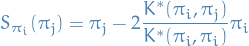
And
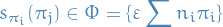
Which means that both terms on LHS of  must be the same sign, and further because it's an element in , we know the coefficient must be in the integers (for
  ):
):
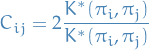
where, for , we have  .
.
Observe,  is not symmetric.
We call the matrix defined by the Cartau matrix, and observe that  while every other entry is some non-positive number!
Now we define the bond number:
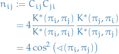
which implies

where and  are non-positive numbers, hence:
Therefore:
|
|
 |
|---|---|---|
| 0 | 0 | 0 |
| -1 | -1 | 1 |
| -1 | -2 | 2 |
| -2 | -1 | 2 |
| -1 | -3 | 3 |
| -3 | -1 | 3 |
Which further implies that

Dynkin diagrams
We draw these diagrams as follows:
for every fundamental root draw circle:

if two circles represent
, draw lines between them:
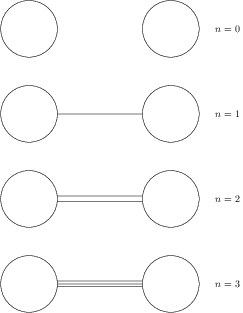
- if there are 2 or 3 lines between two roots, use the
 sign on the lines between to indicate which is the greatest root
Any fininte-dimensional simple - Lie algebra can be reconstructed from the set of fundamental roots and the latter only comes in the following forms:
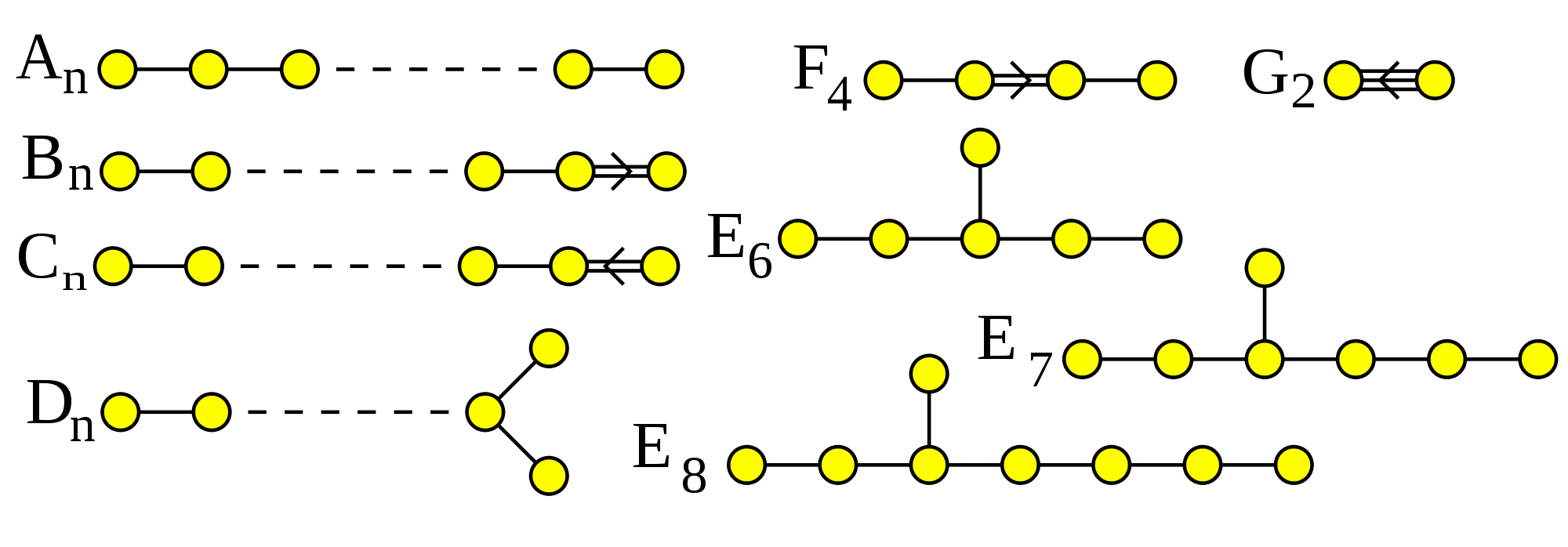
Taken from [[https:/commons.wikimedia.org/wiki/]] /
Representation Theory of Lie groups and Lie algebras
Representation of Lie Algebras
Let ![$\big( L, [\![ \cdot, \cdot ]\!] \big)$](../../assets/latex/geometry_579b92453e8eadcab2e0900fdc549402e995ce4f.png) be a Lie algebra.
be a Lie algebra.
Then a representation  of this Lie algebra is:

(in the Interactions of Algebra, Geometry and Topology course we specific that it should be  rather than
  , since contains inverses)
s.t.
![\begin{equation*}
\varrho \big( [\![ a, b ]\!] \big) = \comm{\varrho(a)}{\varrho(b)} = \varrho(a) \circ \varrho(b) - \varrho(b) \circ \varrho(a)
\end{equation*}](../../assets/latex/geometry_03994e59ecbe19a885493c7cd0eeffa557ebbf6f.png)
where the vector space (a finite-dimensional vector space) is called the representation space.
A morphism between representations and of a Lie group is a linear map  such that

We denote the space of morphisms between Lie group representations and by

A morphism between representations and of a Lie algebra is a linear map such that

We denote the space of morphisms between Lie algebra representations and by

A representation of a Lie group contains the same "data" as an action of the Lie group on a vector space .
Representations of Lie algebra are often called modules over or  .
.
Morphisms between representations are often referred to as intertwining operators.
An example of a representation is
acts on , then
is a representation of via
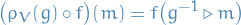
In general,  is an equiv. class of curves where
  if
if  and
and  .
.
are manifolds,  with
with  . Then takes curves through to curves through , and

And takes equiv. classes to equiv. classes (CHECK THIS). Thus differential of ,  .
.
A representation  is called reducible if there exists a vector subspace
  s.t.
s.t.

in other words, the representation map restricts to

Otherwise,  is called irreducible or simple. In other words, if has no non-trivial subrepresentations (i.e. other than 0 or itself).
Example of irreducible representation
The vector representation  of
of  is irreducible.
Irreducible representations
Finite-dimensional reps. of  [EXAM IMP]
First we make the following observation:
- Complex reps. of are isomorphic to those of its real form

- Reps. of are the same as the reps. of

- is compact, thus it's reps. are completely reducible.
- Hence reps. of are iso. to completely reducible reps. reps. are completely reducible, as claimed.
Recall that the generators of satisfy the relations

Let be a representation of with rep.  .
.
A vector is said to be a vector of weight if

i.e. is an eigenvalue of  .
.
We denote ![$V[\lambda]$](../../assets/latex/geometry_1dfebe12ed9ad168d89c90c074ec4df34bb26804.png) the subspace of vectors of weight .
the subspace of vectors of weight .
Note that
![\begin{equation*}
\varrho_V(e) V[\lambda] \subset V[\lambda + 2] \quad \text{and} \quad \varrho_V(f) V[\lambda] \subset V[\lambda - 2]
\end{equation*}](../../assets/latex/geometry_72331f0d3def3d9247b7e3d3ef710729f4815f85.png)
To see this, let ![$v \in V[\lambda]$](../../assets/latex/geometry_58457fc01f75919775891d0c67169a2144796d1c.png) and observe that
and observe that
![\begin{equation*}
\varrho_V(h) \Big( \varrho_V(e) v \Big) = \Big( \underbrace{\comm{\varrho_V(h)}{\varrho_V(e)}}_{= 2 \varrho_V(e)} + \varrho_V(e) \varrho_V(h) \Big) v = \underbrace{(2 + \lambda) \big( \varrho_V(e) v \big)}_{ \in V[\lambda + 2]}
\end{equation*}](../../assets/latex/geometry_0c56a2559da9ccb688525a5bb88e9b01d8a323de.png)
since . Observe then that this means that ![$\varrho_V(e) v \in V[\lambda + 2]$](../../assets/latex/geometry_1e1ee4714fe9a0af674c8b51820f8a85dddd81b4.png) .
.
Similarily we also find that ![$\varrho_V(f) V[\lambda] \subset V[\lambda - 2]$](../../assets/latex/geometry_c3c0781802762fd5abeb12051d239a151ed8e110.png) , as claimed above.
, as claimed above.
Every finite-dimensional rep. of admits decomposition into the weight subspaces:
![\begin{equation*}
V \simeq \bigoplus_{\lambda_i} V[\lambda_i]
\end{equation*}](../../assets/latex/geometry_f98a70b61803b407c0f9fe6cefba918b19aa10a5.png)
Let be a rep. of .
Since reps. of are semi-simple, we can assume to be irreducible.
Let  be the subset spanned by eigenvectors of . By Remark remark:generators-of-sl-2-C-takes-us-from-weight-space-to-weight-space we know that this space is stable under
  and
and  . Hence is a subrepresentation, contradicting the irreducibility of . Therefore
  .
.
Let be a rep. of with  .
.
A weight is said to be a highest weight of if, for any other weight  , one has

Then are called highest weight vectors.

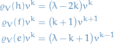
Follows immediately from the fact that
![\begin{equation*}
e V[\lambda] \subset V[\lambda + 2] = 0
\end{equation*}](../../assets/latex/geometry_38d921a71af8a89ca4972ff02b181cbfad2b7646.png)
since
is finite-dimensional and is highest-weight.
- We have the following:
- Action of on
 follows immediately from the def. of .
 - For it follows from the relation
 .
. - For we use induction:
Base step:

General case:
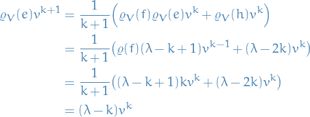
- Action of
For any  , let
, let  be the
  dimensional space with basis
 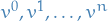 .
.
Define the action of on by
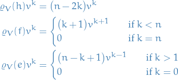
where ![$v \in V[n]$](../../assets/latex/geometry_b0ae59139977134b9942f97372baf4ec34fd1cb4.png) is a highest-weight vector and
is a highest-weight vector and
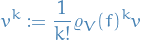
- Then is an irreducible rep. of , it is referred to as the irreducible rep. with highest-weight .
- For any
 we have
- Every finite-dimensional irreducible representation of is isomorphic to for some
 .
.
For any
, we can find an integer such that

Then
 is proportional to
  . Since generates the whole of under action of , we see that is irreducible.
- Since rep.
 and are different dimensions and therefore cannot possibly be isomorphic.
 Let
 and consider an infinite-dimensional representation of
  with the basis
  and the action of defined as before.
Any irreducible finite-dim. rep. which contains highest weight is a quotient of by certain subrepresentation. Let be such a finite-dim. subrep. of . Note, that only finitely many are non-zero in , since all of them are linearly independent. Let be the maximal integer such that
and the action of defined as before.
Any irreducible finite-dim. rep. which contains highest weight is a quotient of by certain subrepresentation. Let be such a finite-dim. subrep. of . Note, that only finitely many are non-zero in , since all of them are linearly independent. Let be the maximal integer such that  . Then

since
 , from which we derive that
  .
Now consider a subspace
.
Now consider a subspace  spanned by vectors
  with
with  . Then is closed under the action of , and hence
  is a subrep. Now it is easy to see that
 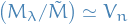 .
.
Then we can consider an infinite dimensional rep. , and quotient by some subrep
In the quotient, there is a "last" vector , which is not killed by  .
.
Take  , then
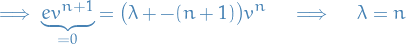
![\begin{equation*}
V = \bigoplus_k n_k V_k = \bigoplus_r V [r]
\end{equation*}](../../assets/latex/geometry_afc552311e648e0f78ca6a537a54e9c5429d6f78.png)
where ![$V[r]$](../../assets/latex/geometry_d2d198865433fdd61d2e8de528d64cd1a75ed303.png) denotes eigenspace of "weight" (with weight referring to the eigenvalue).
This implies that
denotes eigenspace of "weight" (with weight referring to the eigenvalue).
This implies that
![\begin{equation*}
V = \left\{ v^0, \dots, v^n \right\} = : V_n = \underbrace{V_n[n]}_{= \mathbb{C}(v^0)} \oplus \underbrace{V_n[n - 2]}_{\mathbb{C}(v^1)} \oplus \cdots \oplus \underbrace{V_n[ - n]}_{ = \mathbb{C}(v^n)}
\end{equation*}](../../assets/latex/geometry_bb1e73f0a6a74364ee853bb20d59f7891bb0488f.png)
where ![$V_n[k]$](../../assets/latex/geometry_8af3549ef61f67cb21d7bfcdc55e24e304e3cfdb.png) is the h-eigenspace (in ) of weight (which is same if we drop the subscript )
is the h-eigenspace (in ) of weight (which is same if we drop the subscript )
![\begin{equation*}
\dim \big( V[k] \big) = \dim \big( V[-k] \big)
\end{equation*}](../../assets/latex/geometry_d28c613d08209d3474b59cc7cdd5a80f248fcc48.png)
and we get isomorphisms
![\begin{equation*}
V[k] \overset{\overset{f^k}{\longrightarrow}}{\underset{e^k}{\longleftarrow}} V[-k]
\end{equation*}](../../assets/latex/geometry_16060d851dc3893a999425e97c621fcf2d663fd6.png)
 is the std. 2-dimensional
  , then

where  is irreducible of dim.
  .
.
Let

then the character is given by
![\begin{equation*}
\chi_V(t) = \sum_{k}^{} \dim \big( V[k] \big) z(t)^k
\end{equation*}](../../assets/latex/geometry_c35170851bd5d1da39e4ae1fe659562542b39646.png)
where we let  . For some we have
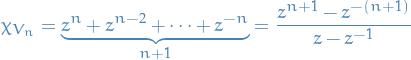
Finite-dimensional rep. theory of is controlled by symmetric functions in  modulo
  .
.
In fact:
Finite-dimensional rep. theory of  is controlled by symmetric functions in
 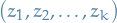 modulo
  .
.
This follows from Lemma lemma:properties-of-character, by taking the tensor products.
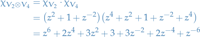
Sanity check at this point: make sure the coefficients sum to the dimensionality of the space!
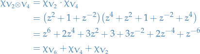
Hence

Say , with eigenvalues in a complex representation are  .
Eigenvalues of in
.
Eigenvalues of in  (
( ) are products
  for
for  (
( )
)

Then

and


Using the above, we have
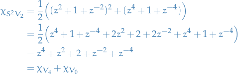
Hence
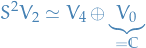
Adjoint representation
Let be a Lie algebra over a field .
Given an element of a Lie algebra , one defines the adjoint action of on is given by the adjoint map.
Then there is a linear mapping
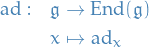
Within  , the Lie bracket is, by definition, given by the commutator of the two operators:

Using the above definition of the Lie bracket, the Jacobi idenity

takes the form

where , , and  are arbitrary elements of .
This last identity says that  is a Lie algebra homomorphism; i.e. a linear mapping that takes brackets to brackets. Hence is a representation of a Lie algebra and is called the adjoint representation of the algebra .
Casamir operator
Let  be the representation of complex Lie algebra .
We define the ρ-Killing form on as
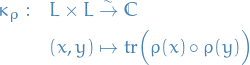
/Note that this is not the same as the "standard" Killing form, where we only consider  .
.
Let be a faithful representation of a complex semi-simple Lie algebra .
Then  is non-degenerate.
Hence induces an isomorphism  by
by

Recall that if  is a basis of , then the dual basis
 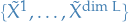 of
of  which is defined by
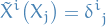
By using the isomorphism induced by (when is a faithful representation, by proposition:ρ-killing-form-induces-isomorphism-for-complex-semi-simple-algebras), we can find some  such that we have
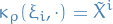
or equivalently,

We thus have,
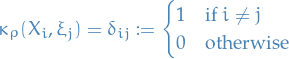
 and
and  be defined as above. Then
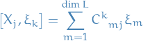
 are the
Let be a faithful representation of a complex (compact) Lie algebra and let be a basis of .
The Casimir operator associated to the representation is the endomorphisms 
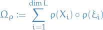
Let  be the Casimir operator of a representation .
Then
that is, commutes with every endormorphism in  .
.
If is irreducible, then any operator which commutes with every endomorphism in , i.e.

has the form

for some constant  (or , if is a real Lie algebra).
Or equivalently, if and are two irreducible complex representations of , then
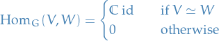
Observe that if we let in the second, we recover the first statement.
For any  , one has that

and

are subrepresentations.
Since both and are irreducible, we conclude that either

In other words, either  or is an isomorphism.
Thus, for  we have
  .
.
Now, if  , the operator is an isomorphism and thus invertible. Let be an eigenvalue of . On one hand,
  is still an intertwining operator, on the other it is not invertible anymore and thus
  . Hence
  .
.
The Casimir operator of is

where
The first part follows from Schurs lemma and Thm. thm:casimir-operator-representation-of-lie-algebra.
The following follows immediately from Schurs lemma.
Let be a completely reducible representation of Lie group or Lie algebra .
Then
 where are irreducible pairwise non-isomorphic representations.
Every intertwining operator
has the form
for some
For 1), notice that any operator  can be written in block form
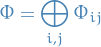
with 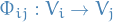 .
By Schur's lemma,
.
By Schur's lemma,  for and
 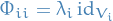 .
.
Part 2) is proven similarily.
Note that Corollary corollary:4.25-kirillov can be quite useful:
- if we can decompose a representation into irreducible representations, this gives us a very effective way of analysing intertwining operators
- For example, if
 with
with  , then
 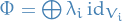 so one can find
  by computing
  for just one vector in .
 - It can also show that each eigenvalue will appear with multiplicity equal to

If is a commutative group, then any irreducible complex representation of is one-dimensional.
Similarily, if is a commutative Lie algebra, then any irreducible complex representation of is one-dimensional.
Complete reducibility of unitary representations
Notation
 denotes the set of isomorphism classes of irreducible representations of
 Matrix coefficients of a representation
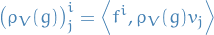
Unitary representations
A unitary representation of a real Lie group (resp. Lie algebra ) is a complex vector space together with a homomorphism  (resp.
  .
.
Equivalently, is unitary if it has a  (resp.
  ) inner product.
Every unitary representation is completely reducible..
If is irreducible, we're done.
If has a subrepresentation , let  be the orthogonal complement of the latter. Then
and is a subrep. as well.
Indeed, if  for any
  , then
We simple iterate the above argument until we're done, i.e. reached  .
.
Every representation of a finite group is unitary.
Let be a rep. of a finite group , and let  be some inner product on .
If is , we are done.
If not, we "average" over in the following fashion: define
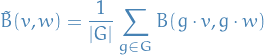
Thus This defined  is positive-definite Hermitian form (because it is a sum of such forms) and is clearly :

Every rep. of a finite group is completely reducible.
Follows directly from thm:every-rep-of-finite-group-is-unitary and then thm:every-unitary-representation-is-completely-reducible.
Haar measure on compact Lie groups
- Idea is to generalize the "averaging" technique from Theorem thm:every-rep-of-finite-group-is-unitary to generalize to infinite Lie groups
A (right) Haar measure on a real Lie group is a Borel measure  which is invariant under the right action of on itself.
Similarily, one defines a left Haar measure.
Let be a one-dimensional real representation of a compact Lie group . Then

Suppose for the sake of contradiction that  , then

On the other hand,  is a compact subset of
  , therefore cannot contain a sequence tending to 0 (since
  and a compact subspace contains all its limit points).
Similar argument shows that  leads to a contradiction as well (just consider inverse of ).
Let be a real Lie group. Then
- is orientable, and the orientation can be chosen so that it is preserved by the right action of on itself.
If
is compact, then for a fixed choice of right-invariant orientation on , there exists a unique right-invariant top-form such that

The form
is also left-invariant and satisfies

- Choose a nonzero element in
 where
where  . Then, it can be uniquely extended to right-invariant top form
  on . Since this form is non-vanishing on , it shows that is orientable.
 If
is compact, we have a finite integral, i.e.

Defining
 we obtain a right-invariant top form satisfying
  . The uniqueness follows from the identification of the space of right-invariant top forms with and the fact that the latter is 1-dimensional. Therefore, any right-invariant form
  for some and the condition
  forces
  .
.
To prove that
is also left-invariant, it is sufficient to show that it is  . The result then follows from the fact that is one-dimensional and Lemma lemma:4.35-kirillov-real-rep-of-compact-Lie-group-has-unit-length.
Finally, let us notice that since is left-invariant, the form
. The result then follows from the fact that is one-dimensional and Lemma lemma:4.35-kirillov-real-rep-of-compact-Lie-group-has-unit-length.
Finally, let us notice that since is left-invariant, the form  is right-invariant, and therefore,

It is clear that
 is given by
  , thus on
  , we have

Choosing the orientation on and the bi-invariant volume form as in Theorem thm:4.34-kirillov, there exists a unique Borel measure on such that for any continuous function on , one has
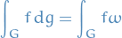
Let be a compact real Lie group.
Then it has a canonical Borel measure, which is both left- and right-invariant under the involution  , and satisfies

This measure is called the Haar measure on .
Any finite-dimensional representation of a a compact Lie group is unitary and thus completely reducible.
Consider a positive-definite inner product  on and "average" it over :
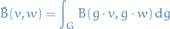
wher is the Haar measure on . Then  as an integral of a positive function, and
  since the Haar measure is right-invariant. Therefore, any finite dimensional representation of a compact Lie group is unitary.
Characters
Now know that any finite-dim rep.
of a compact Lie group is completely reducible, that is
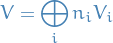
for some irreducible reps.
and positive integers , let's consider how we can find the multiplicities
- For this we need character theory
- Fix a compact Lie group together with a Haar measure
Let
 be non-isomorphic irreducible reps. of and
  . Then
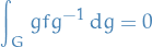
If
is an irreducible repr. and  , then
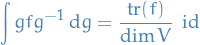
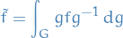
 commutes with the action of
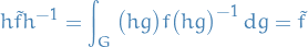
 if
if 
 for
for  . Since

Let be a representation of with a basis  and
and  be a dual basis of ; that is,
Matrix coefficients are functions on of the form
If one writes  as a matrix,
  represents
  entry; hence the name.
Let
be non-isomorphic irreducible reps. of . Choose bases  for and
  for .
Then for any
for .
Then for any  the matrix coeffs.
  and
and  are orthogonal:
where
 is an inner product on
  given by

Let
be an irreducible rep. of and let  be an orthonormal basis wrt. inner product (which exists, as seen before). Then
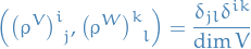
Choose a pair of indices
 and apply Lemma lemma:4.42-kirillov to the mapping
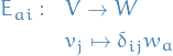
Then, we have
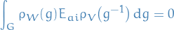
Rewriting the above equality in matrix form and using the unitarity of
 ,
, 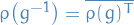 , we obtain for any
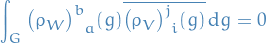
This proves it for orthonormal bases; the general case follows immediately.
Apply Lemma lemma:4.42-kirillov to the matrix unit
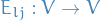 to obtain
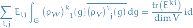
concluding our proof.
A character of a representation is a function on the group defined by
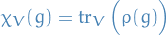
Let
 be a trivial representation. Then

Character of
 :
:

Character of tensor product

Characters are class functions:
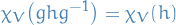
Let
be the dual representation of . Then

Let be irreducible representations of a real Lie group . Then
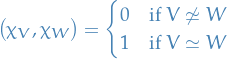
In other words, if denotes the set of isomorphism classes of irreducible representations of , then  is an orthonormal family of functions on .
A representation of is irreducible if and only if
On the other hand, if is semi-simple, and its decomposition into irreducibles reads  , then the multiplicities can be extracted by the following formula
From def:matrix-coefficients-Lie-theory, the matrix coefficients admits a basis-independent definition, namely for ,  , we set
then

where  are dual bases in and . Therefore, for any rep. of we obtain a map
 has additional structure:
- It is a
 , i.e. admits two commuting actions on , those on two tensor factors
 - If is unitary, then the inner product on defines an inner product on
We then define an inner product on by

Let be the set of isomorphism classes of irreducible representations of .
Define the map
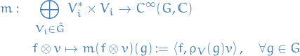
where  is the space of finite linear combinations. Then
The map
is a morphism of  :
:
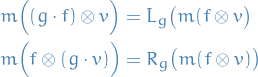
where
 and
and  are the left- and right-actions of on , respectively.
The map
respects the inner product, if it is defined by
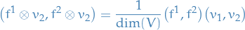
on
 , and on the
  by the formula from the previous lecture:
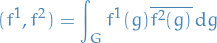
- Follow immediately from the orthogonality theorem from before.
Follows by direct computation:
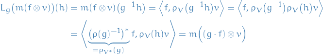
and

as wanted.
is injective.
This follows immediately from the respecting the inner product.
The map in Theorem thm:120-lectures defines an isomorphism
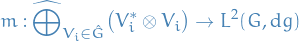
where
 is the Hilbert space direct sum, i.e. the completion of the algebraic direct sum wrt. the metric given by inner product
 is the Hilbert space of complex-valued square-integrable functions on wrt. the Haar measure, wrt. inner product
The set of characters  is an orthonormal basis (in the sense of Hilbert space) of the space
  of conjugation-invariant functions on .
Example: 
- The Haar measure on is given by
 and the irreducible representations are parametrized by
For any
, we have a 1D rep.  with the action of given by
Corresponding matrix coefficient is the same as character, and is given by

Therefore, the orthogonality relation is given by
which is the usual ortogonality relation for exponents.
- Peter-Weyl theorem in this cases just says that the exponents
 for
for  form an orthonormal basis of
  , which is one of the main statements of the theory of Fourier series!
Every
 function
  on can be written as a series
which converges in the
metric.
- For this reason, the study of the structure of
 can be considered as a generalization of harmonic analysis!
Pretty neat stuff, if I might say so myself.
Representation of Lie groups
A representation of a Lie group  is a Lie group homomorphism

for some finite-dimensional vector space .
Recall that  is a Lie group homomorphism if it is smooth and

Let be a Lie group. For each , we define the Adjoint map:
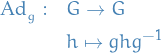
Notice the capital "A" here to distinguish from the adjoint map of a Lie algebra.
Since  is a composition of a Lie group, then it's a smooth map. Further,

Thus,  yields a representation of with
 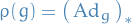 .
Thus,
.
Thus, 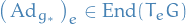 , i.e. it yields a representation of on
  .
.
Consider the following map
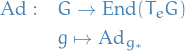
where 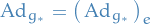 since we are in .
Then

as operators on , where  is the adjoint map of the Lie algebra. To make it explicit, this means

By definition of  we have
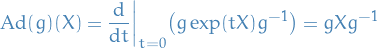
Thus,  is defined as
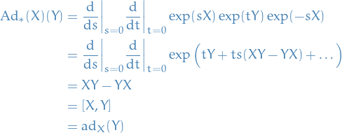
 is a group homomorphism.
Let  and
and  , then

Moreover, the image of  is invertible endomorphisms, i.e. automorphisms since if , then
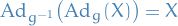
which holds for all .
Lie algebra of vector fields
Stabilizers and centers
Let
 be a morphism of Lie groups
 be the corresponding morphism of Lie algebras
Then
 is a closed Lie subgroup with Lie algebra
  , i.e.

- The map
 is an immersion.
Furhermore, if  is a (embedded) submanifold adn thus a closed Lie subgroup, we have a Lie group isomorphism

Let be a represention of Lie group , and .
Then the stabilizer
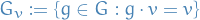
is a closed Lie subgroup in with Lie algebra

Example 3.32 in Kirillov: WRITE IT OUT
Let be a Lie algebra. The center of is defined by

 is an ideal in .
Let be a connected Lie group. Then its center  is a closed Lie group with Lie algebra .
If is not connected, then is still a closed Lie subgroup; however, its Lie algebra might be "smaller" than .
If and  , then
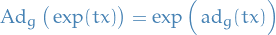
Since is connected, then by 

implies

and

Let be connected.
The Adjoint group

Examples:
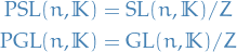
TODO When or  , when
  ?
?
Fundmental Theorems of Lie Theory
- All Lie groups has a canonical structure of a Lie algebra on
 .
.
- For every morphism of Lie groups , we have .
- Moreover, if is connected then
 is injective.
 - Q: When is it also surjective?
- and
 then
then

Consider the identity map
 .
Is there a morphism
.
Is there a morphism  which is locally
  ?
?
- A: NO! Suppose it exists, then it should be given by
 ; on the other hand, it must also satisfy
  . This, this morphism of Lie algebras can not be lifted to a morphism of Lie groups.
- A: NO! Suppose it exists, then it should be given by
- For every morphism of Lie groups
- Every Lie subgroup defines a Lie subalgebra
 .
.
- Q: Does every Lie subalgebra come as
 for some subgroup ?
- A: For any Lie group there is a bijection between connected Lie subgroups and Lie subalgebras.
- A: For any Lie group
- Q: Does every Lie subalgebra come as
- Given a topology of a Lie group, its group law can be recovered from commutator.
- Q: To which extent can we recover the topology?
Any real or complex Lie algebra, is isomorphic to an algebra of some Lie group.
For any real or complex finite-dimensional Lie algebra , there is a unique (up to isomorphism) connected, simply-connected Lie group (respectively, real or complex) with

Moreover, any other connected Lie group  with
with  , i.e. same Lie algebra, must be of the form
  for some discrete central subgroup
  , and is a universal cover of .
By Lie's 3rd theorem, a Lie group s.t.  .
Then just let be the universal cover of the connected component of containing .
Suppose is connected, simply-connected, and .
Then the morphism
.
Then just let be the universal cover of the connected component of containing .
Suppose is connected, simply-connected, and .
Then the morphism  lifts to
  which is locally an identity is discrete is a covering space of so

Complexification / Real forms of Lie algebras and Lie groups
Complexification
Let be a real Lie algebra.
The complexification of is the complex Lie algebra

where  as usual.
The bracket on  induced by
  by
by 
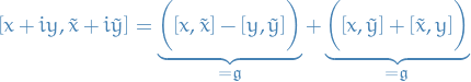
Conversely, we say that is a real form of .


 then
then 
 :
:
 then
then 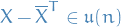
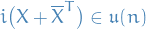
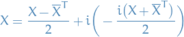
 we ?
we ?Real form
Let be a connected complex Lie group with  .
.
A real form of is a closed real Lie subgroup  s.t.
s.t.

is a real form of .
 there exists a
 - Examples
 is compact real form
- Lie algebras of
 , and
, and 
has a basis
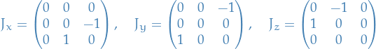
with commutation relations
 have basis
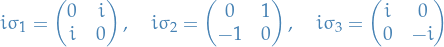
which commutation relations
 has basis
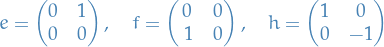
with commutation relations

The isomorphism
 is defined by

Since we saw earlier that
 , we can argue from this that is a complexification of , i.e.
  , where we have the additional constraint of the matrices being traceless. The explicit isomorphism
  is defined

Finally, the isomorphism
 is given by
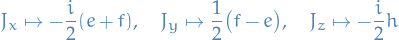
Representations
Let be some  with
with  .
.
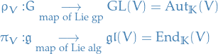
A representation is a pair  .
.
And given two representations and  a morphism of representations is a linear map s.t. the following diagram commutes:
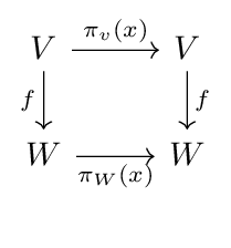
is Lie group with
Every
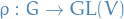 lifts to a
  by
by  .
Moreover,
.
Moreover,

If
is connected and simply-connected, then

which is equivalent to saying that the category of G-representations is equal to the category of
representations.
Let be a real Lie algebra, and be its complexification. The any complex representation of has a unique structure of representation of , and

In other words, categories of complex representations of and are equivalent.
This tells us that if you want to work with complex vector spaces, then there is no reason to work with a real form rather than using the complex version, since they are equal (and over a complex vector space, it's easier to work with complex Lie algebra).
 for any
  for any


Operations on representations
Let be a representation of a Lie group .
A subspace is called a suprepresentation of if it's stable under the action by  , i.e.

Let be a representation of a Lie algebra .
A subspace is called a subrepresentation of if it's stable under the action by  , i.e.

Let be a representation (of group or algebra) and a subrepresentation (of group or algebra).
Then the quotient space  carries a structure of a representation and is called the factor representation or the quotient representation.
Let be a connected Lie group with a representation .
Then is a subrep. for if and only if is a subrep. for
Let be representations of (respectively, ).
Then there is a canoncial structure of a representation on
- : let
 denote the adjoint of an operator , then we have the following reps.:
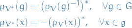
- :
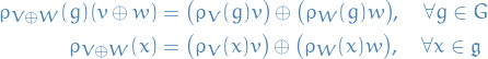
 :
:
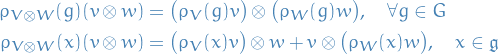
Let and be a "curve" (one-parameter subgroup) such that  .
.
Let
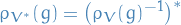
where for an operator
we denote the adjoint . Observe then that this preserves the natural pairing between and  :
:

The corresponding map for the Lie algebra is obtained by simply taking th derivative of some integral curve:
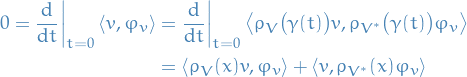
by the product rule. Therefore,

Which implies that
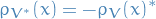
i.e. the adjoint of
.
Since
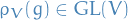 , we simply define the representation on by the linearisation of the action on and respectively. That is, if and ,

Due to the linearity of
, the Lie algebra rep. is identitical (since the derivative-operator is linear):

The group rep. on
is simply

But the algebra rep. is slightly more tricky. A naive approach would be to define it similarily as the group rep. but this does in fact not define a reresentation (it is not even linear in
!). We again consider the derivative of  :
:
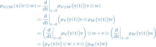
where we made use of the Leibniz rule.
Following Lemma lemma:4.10-kirillov-canonical-representations-of-dual-direct-sum-and-tensor-product we immediately have a canonical representation on the tensor space
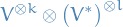
The coadjoint representation of a Lie group and its Lie algebra is the dual vector space  together with the following actions of and respectively:
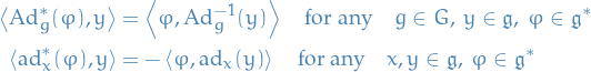
Let be a representation of or .
The space  is naturally a representation of and , respectively. More precisely, we have
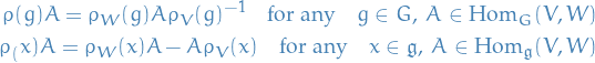
which easily follows from the derivative of a one-parameter subgroup .
Let be a representation of or , respectively.
Then the space of bilinear forms on is a representation as well:
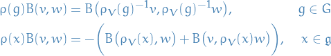
Let be a Lie group with Lie algebra and representation .
Then a vector is called if
The subspace of all vectors is denoted  .
.
Similarily, is called if
The subspace of all vectors is denoted  .
.
If is a connected Lie group, then the the and vector spaces are equal, i.e.

In general, one can easily see that  , since
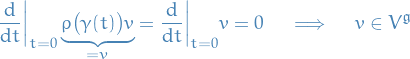
since is just a constant…
Let be  , then

In particular, considering as a trivial one gets

Reconstruction of Lie group from it's Lie algebra
Notation
 denotes the
  map restricted to the vector space
Stuff
is a smooth manifold and be is a smooth vector field on .
Then a smooth curve

is called an integral curve if

There is a unique integral curve of through each point of the manifold .
This follows from the existence and uniqueness of solutions to ordinary differential equations.
Given any  , and any , there exists and a smooth curve
 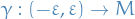 with
with

The maximal integral curve of through is the unique integral curve 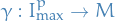 of through , where

So we're just taking the "largest" interval for which there exists integral curves "locally" for .
In general,  differ from point to point for a given vector field .
An integral curve of a vector field is called complete if its domain can be extended to  .
.
Using the definition of maximal integral curve, we say a vector field is complete if  for all .
On a compact manifold, every vector field is complete.
Every left-invariant vector field on a Lie group is complete.
Let  and define the thus uniquely determined left-invariant vector field :

Then let 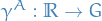 be the integral curve of (which we can due to this theorem) through the point

This defines the so-called exponential map
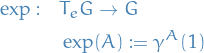
It might be a bit clearer if one writes

Derivative
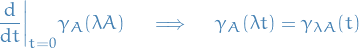
which implies

If
 is a left-invariant vector field implies that time flow along is given by

(and if we replace left-invariant with right-invariant we have
 )
)
Some places you might see people talking about using infinitesimally small generators, say . Then they will write something like "we can generate the group from the generator by expanding about the identity:

where  is our Lie group element generated from the Lie group element !
Now, there are several things to notice here:
- Factor of ; this is just convention, and might be convenient in some cases
- is just what we refer to as
- This is really not a rigorous way to do things…
Finally, and this is the interesting bit IMO, one thing that this notation might make a bit clearer than our definition of is:
- We don't need an expression for
 ; is a smooth curve, and so we can
- Taylor expand to obtain new Lie group element
- new Lie group element
- Goto 1. and repeat until generated entire group
- Taylor expand
Matching with the expression above, only considering first-order expansion, we see that

where
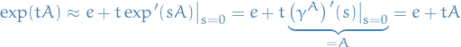
- Neat, innit?!
- is a local diffeomorphism:
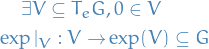
- This restricted map is bijective
 and
and  are smooth
- Follows from IFT
- If is compact then is surjective:
 .
This is super-nice, as it means we can recover the entire Lie group from the Lie algebra!!! (due to this theorem)
However:
.
This is super-nice, as it means we can recover the entire Lie group from the Lie algebra!!! (due to this theorem)
However:
- is non-compact
- is compact
- Hence cannot be injective!
- If is non-compact: it may be not surjective, may be injective and may be bijective.
Just saying it can be whatever if is non-compact.
Letting  .
.
 and
and  by definition
- is a diffeo (as stated above) from a neighborhood of in to a neighborhoud of .
- By IFT has a local inverse, which we call

- By IFT

For any morphism of Lie groups
, we have

This follows from
 being a one-param subgroup in , giving us
has to coincide with

Follows directly from (4):
The ordinary exponential function is a special case of the exponential map when is the multiplicative group of positive real numbers (whose Lie algebra is the additive group of all real numbers).
The exponential map of a Lie group satisfies many properties analogous to those of the ordinary exponential function, however, it also differs in many important respects.
Let be connected, and a morphism of Lie groups.
Then is determined by
connected, hence generated by a neighbourhoud of , i.e. generated by elements  .
But
.
But
Letting  , then if
  are small enough (can expand any analytic function in a sufficiently small neighborhood) we have

because  is close enough to .
Can write
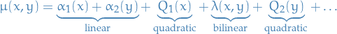
Observe that for the above equation, we let

since  and
and  . Similarily for
  . Thus we see that

And finally, letting  , we see that

From Prop. proposition:expansion-of-exponential-map-in-neighbourhoood-of-identity we can write the commutation in the definition of adjoint map  by
by
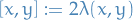
is a Lie group morphism. Then
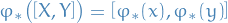 for all
 - Directly from 1):
 for all and all
 Exponential

If is commutative, then so is , i.e.


Due to Theorem thm:baker-campbell-hausdorff we observe that commutators defines multiplication locally.
If is connected, then
- defines

- is commutative is commutative.
- Compare this to corollary:Lie-group-commutative-implies-Lie-algebra-commutative where we have rather than iff, and but in this case is connected, which is not required in the other case.
- Compare this to corollary:Lie-group-commutative-implies-Lie-algebra-commutative where we have
Example
 with Lie algebra
 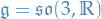 generated by
and
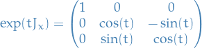
These one-param subgroups generates a neighbourhood of  , and thus by connectedness of
  , it generates the whole of .
 are called "infinitesimal generators".
Flow
A one-parameter subgroup of a Lie group is a Lie group homomorphism

with understood as a Lie group under ordinary addition.
Let be a smooth manifold and let be a complete vector field.
The flow of is a smooth map
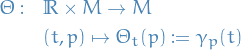
where  is the maximal integral curve of through . For a fixed , we have

For each  the map
  is a diffeomorphism
  . Denoting by
  the group (under composition) of the diffeomorphisms , we have that the map
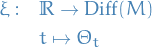
is a one-parameter subgroup of  .
.
Lie group action, on a manifold
Notation
- Unless otherwise specified, assume maps in this section to be continuous
![$[\varepsilon]$](../../assets/latex/geometry_ede670312c6ea3a85074cfc3b28e0b64e9fba037.png) is sometimes used to the denote a specific equivalence class related to the group-element
is sometimes used to the denote a specific equivalence class related to the group-element  denotes the orbit of of the element , i.e.
 denotes the stabilizer of of the element , i.e.
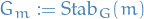
Preparation
Let be a Lie group, and be a smooth manifold.
Then a smooth map

satisfying


is called a left G-action on the manifold .
Similarily, we define a right action:

s.t.


Observe that we can define the right action  using the left action
  :
:
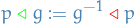
In the literature you might often see the following maps defined as the left action and right action:
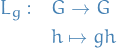
and
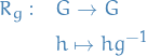
These actions define representations of on vector fields and k-forms on . In particular, for  and
and  we have
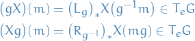
where we've written  for
for  .
.

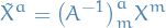
 on the basis
  and a
and a  .
.
Let:
- two Lie group and
 and a Lie group homomorphism
  .
. - and be two smooth manifolds
two left actions
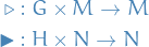
- be a smooth map
Then is called equivariant if the following diagram commutes:
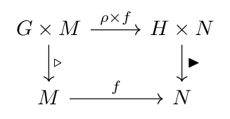
where  is a function where takes the first entry and maps to , and takes the second entry and maps to .
Let  be a left action.
For any
we define it's orbit under the action as the set

Let

which defines a equivalence relation, thus defining a partition of
called orbit space
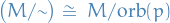
For any
we define the stabilizer

An action  is called free if and only if

where is the identity of the group.
Examples of Lie group actions
 acts on and is a Lie group
 acts on
  since
since
and thus
 we have
- Of course,
 also acts on
- Of course,
 acts on
Classical groups
Let
We use the term classical groups to refer to the following groups:
General linear:

Special linear:

Orthogonal:
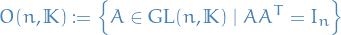
Special orthogonal:

Indefinite orthogonal:

Indefinite special orthogonal:

This group can equivalently be said to be the group of transformations under which a metric tensor with signature
is invariant!
- Ths is why in relativity we consider the group
 (or
(or  depending on the sign-convention being used)!
- Ths is why in relativity we consider the group
Symplectic:

or equivalently

where
is the skew-symmetric bilinear form
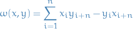
(which, up to a change of basis, is the unique nondegenerate skew-symmetric bilinear form on
 ).
The equivalence of the two above comes from the fact that
).
The equivalence of the two above comes from the fact that 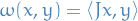 .
.
Unitary:
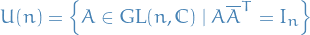
Special unitary:

Unitary quaternionic or compact Symplectic:

Consider for matrices, then  converges for all
  , defined

Furthermore, in some neighborhood of  we have the following series be convergent
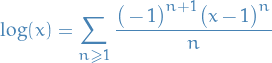
with  .
.
- and are inverse of each other whenever defined.
 and
and 
 implies
 implies
  with around
 the map
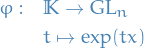
We have
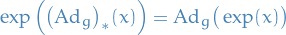
and

then consists of curves whose entries are smooth (or holomorphic) functions in , satisfying  and
and  for all
  , i.e. regular curves. Due to the smoothness, we can write

passing through . This implies that

On the other hand, is a curve in  for any
  , and the corresponding tangent vector is .

From now on, we let
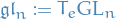
Exercise: For  we have

where multiplication is matrix multiplication. NOTE: this does not make sense in general (i.e. multiplying a group element with elements of tangent space ), but in this case it does, which you can see be looking at the curves, etc.
For all classical  there exists a vector space
  s.t. for a neighbourhood of
  and a neighbourhood of
  where them maps
are mutually inverse.
Each classical group is a Lie group with the tanget space at identity being , where is as in Theorem thm:classical-groups-exp-and-log-mutually-inverse.
If  and with

i.e. and  commute, then we also have

i.e. and  also commute.

Substracting and combining powers,
Suppose now that there exists terms which are non-vanishing and let  be the first indices where we have

Then

so we must have one of the following:
 and
and 
 and
and 
But if 2. is true, then clearly we have all terms vanish, so this cannot be the case. Therefore we must have 1. We can then iterate this argument for both  and
and  until we have
  , i.e. the term

as the first non-vanishing term. But this is under the assumption that all higher order terms are indeed vanishing, the series is simply
But the LHS vanish, and so we must have

as wanted.
G-homogenous space
Let act on , then
- is a closed Lie subgroup of
 is an injective immersion
In particular, is an immersed submanifold in with tangent space

Moreover, if is an (embedded) submanifold, then is a diffeomorphism  .
.
- It's sufficient to prove that in some neighbourhood contained in , the intersection
 is a submanifold with the tangent space
  .
.
Recall that the commutator on vector fields on
, denoted  , can be defined for

Thus the space

is closed under the Lie bracket since
 is a Lie algebra morphism (where we know is in direct correspondance with left-invariant vector fields on )
Also, since the vector field
 vanishes at , we have

where
 corresponds to the flow of with
 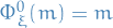 . Therefore

That is, every element of
 exponentiates to .
Choose a vector subspace
 complementary to , i.e.

Since
 , by First Isomorphism Theorem of vector spaces, we know that
  is injective. Therefore the map
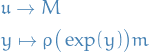
is also injective for "sufficiently small
" (i.e.  near s.t. that the above holds); this is just
  . Therefore

By IFT, any element
in a sufficiently small neighbourhood in can be written as

On the other hand,
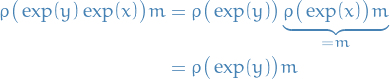
thus

- Since
 is a submanifold in a neighbourhood of , we see that must also be a submanifold (which means that it's a closed Lie subgroup, since when we say submanifold, we mean an embedded submanifold)
The proof of 1) also tells us that there is an isomorphism

so the injectivity of the map
 shows that the map given by
  is an immersion.
A G-homogenous space is a manifold with transitive action of , i.e. 
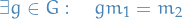
Why is this notation of G-homogenous so useful? Because if acts transitively on , then  for some also acts freely on . From this we then have the bijection
 ![$[g] \mapsto g \cdot m$](../../assets/latex/geometry_302774838c7880d8689c2b9378a9074e9965c191.png) ! Moreover, this map is diffeomorphic
! Moreover, this map is diffeomorphic
If is a G-homogenous space, then there is a fibre bundle  with fibre , where
The proof follows from the fact that we have a diffeomorphism between and following thm:stabilizer-is-closed-lie-group-and-action-diffeomorphism-to-manifold , and we already know that  is a fibre bundle with fibre from earlier.
Let's clarify the above corollary.
If we were to construct a fibration from a group and its action on some G-homogenous manifold we could approach it as follows.
- Let
 be the projection map we are interested in
 - Consider some point , then the corresponding fibre is

Naturally, we must then have
since the action by
 on is identity.
Since
is G-homogenous, i.e. acts transitively, at every point we therefore have
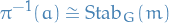
- Results in a fibre bundle
 with fibre (so is a particularly chosen point)
 Since
is transitive, is free, and therefore we have the bijective mapping
![\begin{equation*}
\begin{split}
\varphi_m: \quad & (G / G_m) \to M \\
& [g] \mapsto g \cdot m
\end{split}
\end{equation*}](../../assets/latex/geometry_8c794377ed78b5ebb2537f5eba384b75f711540f.png)
where we write
 to remind ourselves that this bijection depends on the point .
- Need to be diffeo. Since is a Lie group and
Example of application of G-homogenous space

 acts on
  with
with
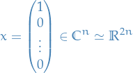
So  has on the first column, and then zeros on the rest of the first row, and then the rest of the matrix is
  . Recall that
  acts as rotation, and so in a basis containing we have
  acting by rotation around the axis .
We get the fibre bundle 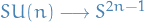 with fibre . We then have the exact sequence

If and  then
then
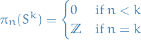
If  , we have
  . This implies

 is a point, hence connected and simply connected, hence so is for all
  !
!
Principal fibre bundles
A bundle  is called a principal G-bundle if
- is a right G-space, i.e. equipped with a right G-action
 is free
- and
 are isomorphic as bundles, where
 , takes a point to it's orbit / equivalence class
Since
is free:
![\begin{equation*}
\rho^{-1} ([\varepsilon]) \cong G
\end{equation*}](../../assets/latex/geometry_873493fa60ff512ede66ec21f091dc5b4239266a.png)
Suppose we have two principal G-bundles:
 under the right Lie group action by
  under the right Lie group action
  by .
by .
Then a principal bundle morphism or map needs to satisfy the following commutation relations:
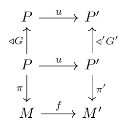
and a further restriction is also that there exists some Lie group homomorphism  , i.e. has to be a smooth map satisfying:

A principal bundle map is a diffeomorphism.
A principal G-bundle under the action by is called trivial if it is diffeomorphic to the principal G-bundle  equipped with
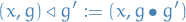
and

That is, is trivial if and only if it's diffeomorphic to the bundle where the total space is the mfd. with attached as the fibre to each point, or equivalently (due to this theorem) if there exists a principal bundle map between these bundles.
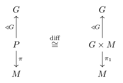

Let be a manifold. First observe that

i.e. the bundle is simply the set of all possible bases of .
The frame bundle is then
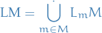
where  denotes the unique union.
Equip  with a smooth atlas inherited from .
Further we define the projection  by
by

which implies that  is a smooth bundle.
Now, to get a principal bundle, we need to establish a right action  on , which we define to be

which is just change of basis, and is therefore free.
Checking that this in fact a principal bundle by verifying that this bundle is in fact isomorphic to  .
.
Observe that the Frame bundle allows us to represent a choice of basis by a choice of section in each neighborhood , with  .
.
That is, any  is a choice of basis for the tangent space at . This is then equipped with the general linear group , i.e invertible transformations, which just happens to be used for to construct change of bases!!!
Ya'll see what this Frame bundle is all about now?
Associated bundles
Given a G-principal bundle (where the total space is equipped with  for ) and a smooth manifold on which we can have a left G-action:

we define the associated bundle

by:
let
 be the equivalence relation:

Thus, consider the quotient space:

In other words, the elements of
 are the equivalence classes
 ![$[(p, f)]$](../../assets/latex/geometry_5c744b271e4ec413de21e3895c0a881957358cbe.png) (short-hand sometimes used
(short-hand sometimes used ![$[p, f]$](../../assets/latex/geometry_99f2d92c746fff9b3ff722eaa06cccc84b7a9842.png) ) where
) where  ,
,  .
.
Define
 by
by
![\begin{equation*}
[p, f] \mapsto \pi(p)
\end{equation*}](../../assets/latex/geometry_fd25fef38fabddb778a7bd70088f4d95df60143d.png)
which is well-defined since
![\begin{equation*}
\pi_F \big( [ p \triangleleft g, g^{-1} \triangleright f ] \big) = \pi (p \triangleleft g ) = \pi(p) = \pi_F \big( [p, f] \big)
\end{equation*}](../../assets/latex/geometry_b8f27ff7ff765a7090fa8f7f050fed1b67260c94.png)
This defines a fibre bundle with typical fibre :
Example of associated bundle: tangent bundle
 which is the frame bundle, and we recall that
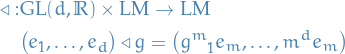

define left action
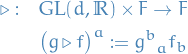
That is, if we change the frame by the right-action (which represents a change of basis), then we must change the components of the tangent space (if we let be the tangent space).
Then  is the associated bundle of the frame bundle.
Example: tensor associated bundle
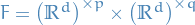
With the left action of on :

Which defines the tensor bundle wrt. some frame bundle  .
.
Observe that we can easily obtain  from using the notion of a dual bundle!
So what we observe here is that "changes of basis" in the frame bundle, which is the principal bundle for the associated bundles tangent bundle and tensor bundle, corresponds to the changes to the tangent and tensors as we are familiar with!
That is, upon having the group  act on the frame bundle, thus changing bases, we also have this same group act on the associated bundles!
Example of associated bundle: tensor densitites
But now, left action of on :

for some  .
.
Then  is called the (p, q)-tensor density bundle over .
Observe that this is the same as the tensor bundle, but with the factor of  in front, thus if we had instead used
  , i.e. orthogonal group, then
  , hence it would be exactly the same as the tensor bundle!
Associated bundle map
An associated bundle map between two associated bundles  (sharing the same fibre, but being associated to arbitrarily different respective G-principal bundle
  )
)
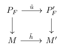
is a bundle map  (structure-preserving map of bundles) which can be costructed from a principal bundle map between the underlying principal bundles,
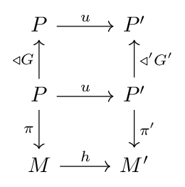
where
as
![\begin{equation*}
\begin{split}
\tilde{u} \big( [p, f] \big) &:= \big[ u(p), f \big] \\
\tilde{h}(m) &:= h(m) \\
\forall p \in P, \ f &\in F, \ m \in M
\end{split}
\end{equation*}](../../assets/latex/geometry_85aee3b7b12ee93613d86dea4660c4185f573179.png)
Restricted Associative bundles
Let
- be a closed subgroup of
- a G-principal bundle over
 a H-principal bundle over
If there exists a bundle morphism (NOT principal) such that
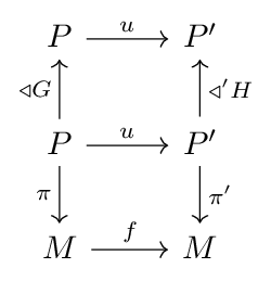
with:

Then
 is called a G-extension of the H-principal bundle
- is called an H-restriction of the /G-principal bundle
i.e. if one is an extension of the other, then the other is a restriction of the one.
Example: vector bundle
A real vector bundle of rank on a manifold (the base space), is a space (the total space) and a projection map  such that
- For every , the fibre
 is a real vector space of
Each
has a neighborhood  and a diffeo.

i.e. a local trivialization, such that
 maps the vector space
  isomorphically to the vector space
On
 , the composition

takes the form

for a smooth transition map
 .
.
Let  be a real rank vector bundle.
We say 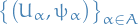 is a trivializing cover with transition maps
  if
if

and  are local trivializations.
The cocycle conditions are that for all  , we have
 for all
 for all
 for all
One can show that a vector bundle satisfy these conditions.
Let
- be a manifold
 an open cover
A collection of smooth maps

satisfying the cocycle conditions
Then there exists a vector bundle with projection map and transition maps  .
.
Define
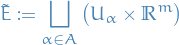
and the equivalence relation

for all  and
and  .
.
Let's check that this is indeed a equivalence relation:
- Clearly
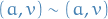 since since satisfy the cocycle conditions
 If
 then
then  such that

since
and  satisfy the cocycle conditions.
- Finally, if and
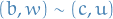 then by satisfying the third condition of the cocycle conditions, we find that this is also satsified.
Hence it is indeed an equivalence relation.
Then we define the quotient space  with the equivalence relation from above, and we define the projection map by
![\begin{equation*}
\begin{split}
\pi: \quad & E \to M \\
& [(a, v)] \mapsto \pi \big( [(a, v)] \big) = a, \quad \forall a \in M, v \in \mathbb{R}^m
\end{split}
\end{equation*}](../../assets/latex/geometry_84e840e092ee9215b8e3e1f4e3c0eb4688443287.png)
where ![$[(a, v)]$](../../assets/latex/geometry_25286255107be9ab5fc64d46847eec49914aa8bd.png) denotes the equivalence class of for some . Then
denotes the equivalence class of for some . Then
![\begin{equation*}
\preim_{\pi} \big( U_{\alpha} \big) = \left\{ [(a, v)] \in E \mid a \in U_{\alpha}, v \in \mathbb{R}^m \right\}
\end{equation*}](../../assets/latex/geometry_ad49e131439279e1c0cce8d3631202c3f2341baa.png)
and we define the map 
![\begin{equation*}
\begin{split}
\psi_{\alpha}: \quad & \preim_{\pi}(U_{\alpha}) \to U_{\alpha} \times \mathbb{R}^m \\
& [(a, v)] \mapsto (a, v)
\end{split}
\end{equation*}](../../assets/latex/geometry_01830372e314dedcc7de307f9add29fbde93312e.png)
Refining (if necessary) the open cover  , we can assume that the are charts, with corresponding chart maps
  (which are also bijections). Then the map

Finally, we observe that 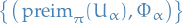 is indeed an atlas for . The charts clearly form a open cover of by definition of
  and the quotient topology, terefore we only need to check that
  are (smooth ?) homeomorphisms to ϕ(Uα)$.
Using Theorem thm:existence-of-vector-bundle-of-manifold we can construct new vector bundles from old ones by using the "functional" constructions ,  , and on vector spaces. The Whitney sum is an example of this.
Let  and
and  be vector bundles of rank
  and , respectively.
Then we define  to be the vector bundle with fibres
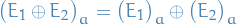
and transition maps
![\begin{equation*}
\begin{split}
g_{\alpha \beta}^{E_1 \otimes E_2}: \quad & U_{\alpha} \cap U_{\beta} \to \GL(k + l, \mathbb{R}) \\
& a \mapsto \left[
\begin{array}{@{}c|c@{}}
g_{\alpha \beta}^E(a) & \\
\hline
& g_{\alpha \beta}^F(a)
\end{array}
\right]
\end{split}
\end{equation*}](../../assets/latex/geometry_c3379c95bfe2f237fc1b81f2f2930dba4bb66abc.png)
where we have used a common refinement  , since we wlog. we can take intersections of the of covers of the two bundles to obtain a new open trivializing cover which is common to both bundles.
One can then see that  are smooth and obey the cocycle conditions as follows. The map
![\begin{equation*}
\begin{split}
\varphi: \quad & \GL(k, \mathbb{R}) \times \GL(l, \mathbb{R}) \to \GL(k + l, \mathbb{R}) \\
& (A, B) \mapsto \left[
\begin{array}{@{}c|c@{}}
A & \\
\hline
& B
\end{array}
\right]
\end{split}
\end{equation*}](../../assets/latex/geometry_a705f2baf770c52f6190944c8e88dc671322005e.png)
is a smooth map on  to
to  . Furthermore, it's a group homomorphism, i.e. it satisfies

Following the example of the Whitney sum, we can obtain the generalized tangent bundle:
Using the Whitney sum we can construct the generalized tangent bundle:

Let  be a rank real vector bundle.
Then consider  , with fibres
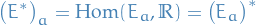
with transition maps  are the inverse transpose of
  . The group homomorphism underlying this is
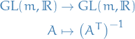
This is a homomorphism since the entries of  are rational functions of entries of and the denominators are
  , which is non-zero in
  !
!
Observe that we can easily obtain from using the notion of a dual bundle!
Let
- and
 be real vector bundles of ranks and , respectively
Then define  is denotes a vector bundle with the typical fibre
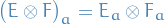
with the transition maps
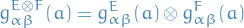
and if  , then

defines a map
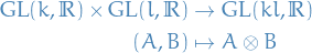
(whose entrires are polynomial in entries of and ).
We can iterate this construction to arrive a  . In particular, we can start with and arrive at the tensor bundle:
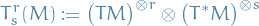
- Examples of vector bundles
- For the tangent bundle , the
 is the Jacobian matrix of a change of coordinates
- So it's really the associated bundle of the frame bundle! We saw this in our previous definition of the associated tangent bundle
- For the cotangent bundle , the
 is the inverse of the transpose Jacobian!
- For the tangent bundle
Connections
Let be a principal G-bundle.
Then each induces a vector field on
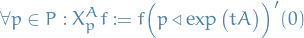
It is useful to define the map
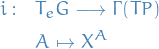
which can be shown to be a Lie algebra homomorphism
![\begin{equation*}
i \Big( [\![ A, B, ]\!] \Big) = \comm{i(A)}{i(B)}
\end{equation*}](../../assets/latex/geometry_392a7fff6ecfec7876eca72cbd6972607dd27a1e.png)
where:
- is the Lie bracket on
- is the commutation bracket on

Let . Then
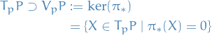
where:
 is the push forward of the bundle projection
 is called the vertical subspace at point .
Idea of a connection is to make a choice of how to "connect" the individual points of "neighboring" fibres in a principal bundle.
Let's take a moment to think about this. For a principal G-bundle we know the fibre at each point is isomorphic to the group . Consider two points in 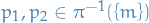 , and
, and  ,
,  . One then wonder how these vectors are pushed down to the manifold at , i.e. what is
  and
and  , both of which lie in . We are then defining
  , the vertical space, as those
  and
and  , in possibly different tangent spaces, are pushed down to the zero-tangent (i.e. the tangent correspondig to the constant path through ).
A connection on a principal G-bundle is an assignment where every for a vector subspace  of
of  is chosen such that
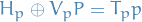 where is the vertical subspace
The push-forward by the right-action of
satisfy:

The unique decomposition:
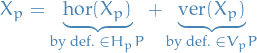
leads, for every smooth vector field
 , to two smooth vector fields
  and
and  .
.
Some principal G-bundle
The choice of horizontal subspace at each , which is required to provide a connection, is conveniently "encoded" in the thus induced Lie-algebra-valued one-form , which is defined as follows:
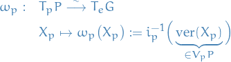
where we need to remember that  depends on the choice of the horizontal subspace !
Recall that  is the map defined in the beginning of this section:
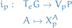
where is called the connection 1-form wrt. the connection.
That is, the connection is a choice of horizontal subspaces of the fibre of the principal bundle, and once we have such a space, we can define this connection 1-form.
Therefore one might wonder "can we go the other way around?":
- Define connection 1-form with certain properties which induces some horizontal space on the principal G-bundle
Yes, we can!

A connection 1-form wrt. a given connection has the properties
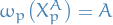
Pull-back
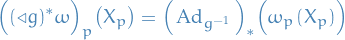
where we recall
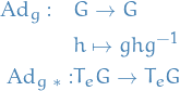
Smooth, since

where
is smooth since the exponential map is smooth.
Different approach to connections
This approach is the one used by Schuller in the International Winter School on Gravity and Light 2015.
A connection (or covariant derivative)  on a smooth manifold
  is a map which takes a pair
  consisting of a vector field and a (p, q)-tensor field and sends this to a (p, q)-tensor field
  , satisfying the following properties:

 for
for 
The Leibnitz rule for
 :
:

and the generalization to a (p, q)-tensor follows from including further terms corresponding to
 of the arguments.
It's worth noting that this is actually the definition obtained from
of the arguments.
It's worth noting that this is actually the definition obtained from
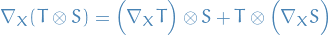
which is the more familiar form of the Leibnitz rule.
 (in )
(in )

Consider vector fields . Then
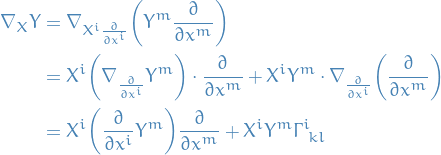
A vector field
on is said to be parallely transported along a smooth curve with tangent vector  if
if

i.e.
A weaker notion is
for some
 , i.e. it's "parallel".
Local representations of connections the base manifold: "Yang-Mills" fields
In practice, e.g. for computational purposes, one whishes to restrict attention to some :
- Choose local section
 , thus
Such a local section induces:
"Yang-Mills" field,
 :
:
i.e. a "local" version of the connection 1-form on the principle fiber
, defined through the pull-back of the chosen section .
Local trivialization ,
, of the principal bundle
Then we can define the local representation of

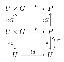
Suppose we have chosen a local section .
The Yang-Mills field , i.e. the connection 1-form restricted to the subspace , is then defined
Thus, this is a "Lie algebra"-valued 1-form.
Choosing the local trivialization :
Then we can define the local representation of the global connection :

given by

where


 is the Maurer Cartan form
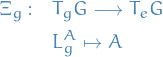
where we have

Examples of Yang-Mills field:
 in Electrodynamics
 in GR, i.e. connection coefficients / Christoffel symbols
Gauge map
- Can we use the "local understading" / restriction to , to construct a global connection 1-form?
- Can do so by defining the Yang-Mills field for different, overlapping subspaces of the base-manifold!
- Need to be able to map between the intersection of these subspaces; introduce gauge map
Suppose we have two subspaces of the base manifold 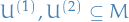 , such that
  for which we also have chosen two corresponding sections
  , such that
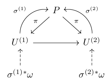
We then define the gauge map as

where is the underlying Lie group (on ), defined on the unique  for all
  :
:
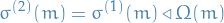
where is the Maurer-Cartan form.

 of
of Example: Frame bundle
Recall that in the case of the Frame budle we have

Then a particular choice of section  for some chart is equivalent of a specific choice of coordinates:
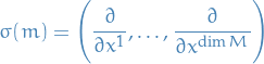
Let's first consider this as an instance of a Yang-Mills field:

is then a Lie-algebra valued one-form on , with components

where
 comes from being a one-form on , hence components
 from
from 
In fact, these are the Christoffel symbols from GR!
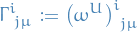
In GR we pretend that all these indices  are related to the manifold , but really the indices
  are related to the Lie algebra (resulting from the Lie group ) while the index is an proper component of the one-form!
We can obtain the gauge map for the Frame bundle. For this we first need to compute the Maurer-Cartan form in  . We do this as follows:
Choose coords an open set
 on
on  containing
  :
:
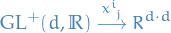
where
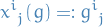
which are the "matrix entries".
We then consider
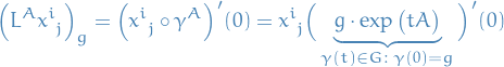
since
 is the unique integral curve of
- by def. of vector-field acting on a map
This can then be written
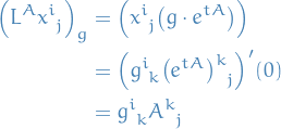
Hence,
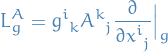
Since
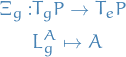
we, in this case, have
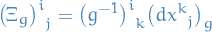
Then,
![\begin{equation*}
\begin{split}
\tensor{\big( \Xi_g \big)}{^i_j} \Big( L_g^A \Big)
&= \bigg[ \tensor{\big( g^{-1} \big)}{^i_k} \tensor{dx}{^k_j}\big|_g \bigg] \bigg[ \tensor{g}{^p_r} \tensor{A}{^r_q} \frac{\partial }{\partial \tensor{x}{^p_q}}\bigg|_g \bigg] \\
&= \tensor{\big( g^{-1} \big)}{^i_k} \tensor{g}{^p_r} \tensor{A}{^r_q} \tensor{dx}{^k_j}\big|_g \frac{\partial }{\partial \tensor{x}{^p_q}}\bigg|_g \\
&= \tensor{\big( g^{-1} \big)}{^i_k} \tensor{g}{^p_r} \tensor{A}{^r_q} \tensor{\delta}{^k_p} \tensor{\delta}{^q_j} \\
&= \tensor{\big( g^{-1} \big)}{^i_k} \tensor{g}{^k_r} \tensor{A}{^r_j} \\
&= \tensor{A}{^i_j}
\end{split}
\end{equation*}](../../assets/latex/geometry_d49af390deff4997d8642cd9f39f6cfc27edd1c6.png)
as we wanted!
Recalling the definition of the gauge map, we now want to compute
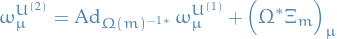
where is the index of the components.
To summarize, we're interested in
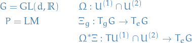
Let 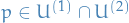 , then
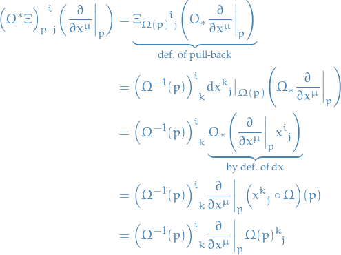
Hence, considering the components of this
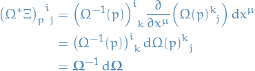
where  denotes the corresponding matrix.
Now, we need to compute the second term:
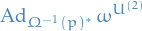
Observe that
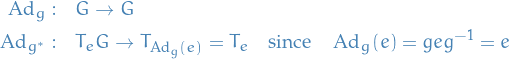
Thus,
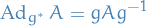
The above can be seen from:

Finally, this gives us the transition between the two Yang-Mills fields
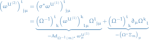
That is, we got it yo!
Structure theory of Lie algebras
Notation
- denotes finite-dimensional Lie algebra over ground field
Universal enveloping algebra
The universal enveloping algebra of , denoted by  , is the associative algebra wih unit over with generators
 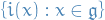 subject to relations
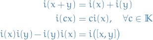
For simplified notation, one will often write  instead of
  , which will be justified later when we show that
  is injective (and so we can consider as a subspace in ).
If we dropped the relation

from universal enveloping algebra, we would get the associative algebra generated by elements with no relations other than linearity and associativity, i.e. tensor algebra of :
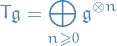
Therefore, we can alternatively describe the universal enveloping algebra as a quotient of the tensor algebra:

Even when  is a matrix algebra, multiplication in is not necessarily std. multiplication of matrices.
E.g. let  , then
  as
as  matrices, but
  in ; there are many representations of in which
  .
.
Let
- be an associative algebra with unit over
 be a linear map such that

Then can be uniquely extended to a morphism of associative algebras  .
.
This is the reason why we call the universal associative algebra.
Any rep. of (not necessarily finite-dim) has a canonical structure of a module.
Conversely, every has a canoncial structure of a representation of .
In other words, categories of reps. of and modules are equivalent.
Example: commutative Lie algebra
Letting be a commutative Lie algebra, then is generated by elements with relations , i.e.

is the symmetric algebra of , which can alos be described as the algebra of polynomial functions n . Choosing a basis  in , we see that
![\begin{equation*}
U \mathfrak{g} = S \mathfrak{g} = \mathbb{K}[x_1, \dots, x_n]
\end{equation*}](../../assets/latex/geometry_80da05cd157aef0705376ae97b47e48e2652a4d1.png)
Example:
Universal enveloping algebra of is the associative algebra over generated by elements , , and with relations
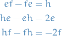
So if say  , then

Hence  is an ideal.
Parallel Transport
This is the proper way of introducing the concept of Parallel transport.
The idea behind parallel transport is to make a choice of a curve ![$\gamma^{\uparrow}: [0, 1] \to P$](../../assets/latex/geometry_f8c616dd4dd7258d4b298f40a5678461153c59bd.png) from the curve in the manifold
from the curve in the manifold ![$\gamma: [0, 1] \to M$](../../assets/latex/geometry_c97bc499b43b6d62051086920b47dc8dabbd97c8.png) , with
, with

Since we have connections between the fibres, one might think of constructing "curves" in the total space by connecting a chosen point  for to some other chosen point
  for
for  , with and
  being "near" each other.
Then the unique curve
![\begin{equation*}
\gamma^{\uparrow}: [0, 1] \to P
\end{equation*}](../../assets/latex/geometry_b8396b87039eb21b8e341e0502d9edf521a3f382.png)
through a point  which satisfies:

 , for all
 ![$\lambda \in [0, 1]$](../../assets/latex/geometry_7cd670af2080b3c73aac2cd9f356000145119694.png)
 , for all
is called the lift of through .
My initial thoughts for how to approach this would be to make a choice of section at each  , such that

where would be a choice for every . Just by looking at this it becomes apparent that this is not a very good way of going about this, since we would have to choose these sections for each such that it's all well-defined. But this seems like a very "intricate" way of going about this.
The idea is to take some such curve as a "starting curve", denoted  , and then construct every other
  from this
  by acting on it at each point by elements of , or rather, choosing a curve
 ![$g: [0, 1] \to G$](../../assets/latex/geometry_82a1002273f9ddf37606533d4c503f95b85e8fac.png) in the Lie-group, such that
in the Lie-group, such that
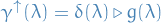
i.e. we can generate any lift of simply by composing the arbitrary curve with some curve in the Lie-group.
It turns out that the choice of is the solution to an ODE with the initial condition

where  is the unique group element such that

The ODE for is

with initial condition
such that
Worth noting that this is a first-order ODE.
Horizontal lift
Let
 be a principal G-bundle and a connection one-form on
  be the associated fibre bundle of whose typical fibre the Lie group acts on the left by
 - be a curve on
 be its horizontal lift to through
Then the horizontal lift of to the associated bundle through the point ![$[p, f] \in P_F$](../../assets/latex/geometry_b362f4a828c2ef4b29d9fe379f9e388b287860e6.png) is the curve
is the curve
![\begin{equation*}
\begin{split}
\overset{\overset{P_F}{\uparrow}}{\gamma}_{[p, f]}: \quad & [0, 1] \to P_F \\
& \lambda \mapsto \big[ \overset{\uparrow}{\gamma}_p(\lambda), \ f \big]
\end{split}
\end{equation*}](../../assets/latex/geometry_d77b2e378f0e95260b39164bb3b1a7e53316e3a4.png)
Curvature and torsion (on principle G-bundles)
Curvature
Let  be a principle G-bundle with a connection 1-form .
Then let be a A-valued (e.g. Lie-algebra valued) k-form, then
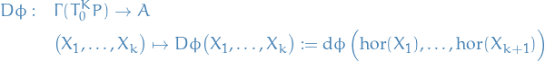
is called the covariant exterior derivative of .
Let be a principal G-bundle with the connection 1-form .
Then the curvature (of the connection 1-form) is the Lie-algebra-valued 2-form on
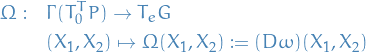
Curvature (of 1-form) can also be written

where in the case Lie-algebras we have
![\begin{equation*}
(\omega \doublewedge \omega)(X, Y) := [\![ \omega(X), \omega(Y) ]\!]
\end{equation*}](../../assets/latex/geometry_1d9cfc823f6406f37ded5aaaeca1055388139cc2.png)
but the  is used to not restrict ourselves to Lie-algebra-valued forms, in which case becomes different.
First observe that  is
is  bilinear.
We do this on a case-by-case basis.
- and are both vertical, i.e.
 . Then

Then

And
![\begin{equation*}
\begin{split}
\text{RHS} &= \big( \dd{\omega} \big)(X^A, X^B) + \big( \omega \doublewedge \omega \big)(X^A, X^B) \\
&= X^A \Big( \underbrace{\omega(X^B)}_{ = B} \Big) - X^B \Big( \underbrace{\omega(X^A)}_{= A} \Big) - \omega \Big( \underbrace{\comm{X^A}{X^B}}_{\overset{(1)}{=} X^{[\![ A, B ]\!]}} \Big) + [\![ \underbrace{\omega(X^A)}_{ = A}, \underbrace{\omega(X^B)}_{ = B} ]\!] \\
&= \underbrace{X^A(B)}_{ = 0} + \underbrace{X^B(A)}_{= 0} - \underbrace{\omega \Big( X^{[\![ A, B ]\!]} \Big)}_{= [\![ A, B ]\!]} + [\![ A, B ]\!] \\
&= 0
\end{split}
\end{equation*}](../../assets/latex/geometry_98da2a16bbc520a3eb964c25f2283ec69b123d28.png)
where at
 we've used the the fact that the map
defines a Lie-algebra homomorphism.
- and are both horizontal, i.e.
 . Then

and
![\begin{equation*}
\begin{split}
\text{RHS} &= \dd{\omega}(X, Y) + \big( \omega \doublewedge \omega \big)(X, Y) \\
&= \dd{\omega}(X, Y) + [\![ \underbrace{\omega(X)}_{= 0}, \underbrace{\omega(Y)}_{= 0} ]\!] \\
&= \dd{\omega}(X, Y)
\end{split}
\end{equation*}](../../assets/latex/geometry_7436b2df584c378b39fbe6f2a356172618365832.png)
since from Remark remark:horizontal-space-as-kernel-of-connection-1-form we know that

(wlog)
is horizontal, and is vertical, i.e.

Since any tangent can be separated into horizontal and vertical component, we know showing these cases is sufficient. Furthermore, since both sides of the expression we want to show is anti-symmetric in the arguments, if
and were swapped we'd pick up a minus sign on both sides which cancel each other out. Then
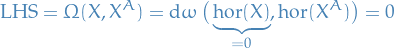
and
![\begin{equation*}
\begin{split}
\text{RHS} &= \dd{\omega} \big( X, X^A \big) + \big( \omega \doublewedge \omega \big)(X, X^A) \\
&= X \big( \underbrace{\omega(X^A)}_{= A} \big) + X^A \big( \underbrace{\omega(X)}_{ = 0} \big) - \omega \big( \underbrace{\comm{X}{X^A}}_{\text{horizontal}} \big) + [\![ \underbrace{\omega(X)}_{ = 0}, \omega(X^A) ]\!] \\
&= \underbrace{X(A)}_{ = 0} + \underbrace{X^A(0)}_{ = 0} - \underbrace{\omega \big( \comm{X}{X^A} \big)}_{ = 0} + \underbrace{[\![ 0, \omega(X^A) ]\!]}_{ = 0} \\
&= 0
\end{split}
\end{equation*}](../../assets/latex/geometry_585e05032d3fd0cf80ed58aff18e2fb845e81a34.png)
where the only thing to "wonder about" is why
 is horizontal, which follows from the fact that:
If is a matrix group, then
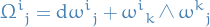
where the is justified since we're summing over the indices and is anti-symmetric, so we end up the equivalent of the std. commutator bracket  used for matrix groups.
Relating to curvature on base space
- Most often the notion of curvature is seen on the base manifold, rather than on the total space, as we saw in the previous section
- In this section we relate the notion of curvature on the total space to curvature on the base space
Consider a section for some , where is equipped with a connection 1-form and corresponding curvature. Then, as we have seen earlier, this choice of section induces
-

where the
and are often seen symbols in Physics.
 denotes the fact that it's a Lie-algebra valued 1-form
Yang-Mills field-strength:

where
 denotes a Riemann tensor and is often used in Electrodynamics
 denotes the fact that it's a Lie-algebra valued 2-form
Observe that on :
and
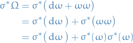
by linearity of the pullback.
Field-strength in Electrodynamics
Observe that the field-strength tensor seen in Electrodynamics
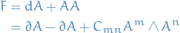
for some coefficients  .
.
Bianchi identity
(which is NOT the same as the ![$\dd[2]{} = 0$](../../assets/latex/geometry_515b05a10ea270c1985da364ec2bbdea0cb1d411.png) , i.e.
, i.e.  in general!!!)
Torsion
Let be a principal G-bundle and let be the representation space of a linear  representation of the Lie group .
A solder(ing) form on is a one-form  such that
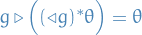
- and
 are isomorphic as associated bundles, where then
  is also a vector bundle.
A solder form provides an identification of with each tangent space of , i.e. each .
Let be a principal G-bundle with connection 1-form and let be a solder form on . Then

defines the torsion of wrt.  .
.
We might want a similar formula as we found for the curvature in Proposition proposition:curvature-rewritten. However, since  and are both V-valued but is valued, the term
  does not make sense. Instead we have

where  denotes the fact that we let act on .
More precisely, in the case of a matrix Lie group, recalling that  , we have
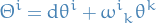

Like and , a torsion two-form can also be pulled back to the base manifold along a local section as  .
.
In fact, this is the torsion that one typically meets in general relativity!
TODO Covariant derivatives
Spinors on curves spaces

 (i.e. inner product), i.e. we can construct a
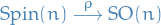


Relating to Quantum Mechanics
Schrödinger:

where

 can be writtein in terms of
  and
and  where we recall
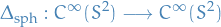
- First need to understand
Idea:
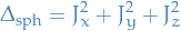
where
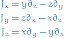
 commutes with
For now, consider  polynomials in
  of at most degree
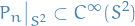
Moreover, is a subrep. of because is generated by .
Relating to the isomorphism between and , we want to diagonlize  . To do so, we make a change of coordinates to cylindrical coords.
Let  denote the basis-elements of .

where


where  form a basis in complexification of .
Let

On  we have
For basis we can take
In this basis, where 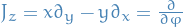 and so
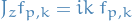
Now consider ![$P_n[2k]$](../../assets/latex/geometry_1e646c54ae2fc5e4e661b0673fd8bbf0f2fe196b.png) , i.e. subspace of with "weights" (eigenvalues)
, i.e. subspace of with "weights" (eigenvalues)  . Then
![\begin{equation*}
P_n[2k] = \mathrm{Span} \left\langle f_{p, k} \mid 0 \le p \le n - |k| \right\rangle
\end{equation*}](../../assets/latex/geometry_313f0cf4204f874e98b5e1a5a58c66cc78e21c04.png)
(as a  ) since we know that we have the isomorphism
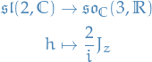
Choosing some  , we have
![\begin{equation*}
\dim \big( P_n[2k] \big) = n - k + 1
\end{equation*}](../../assets/latex/geometry_8481f5e1cc34b8b08baa589f7eb119352975f047.png)

(which we you'll do in assignment)
CORRECTION TO COME: negative eigenvalues? Whattabout dem thingies? Accounted for because symmetry? What…
(Assignment) acts on by 
And so we have diagonlized on polynomials in restricted to .
Complex dynamics
This section mainly started out as notes from the very interesting article by Danny Stoll called "A Brief Introduction to Complex Dynamics" (http://math.uchicago.edu/~may/REUDOCS/Stoll.pdf).
Notation
- denotes a Riemann surface
Definitions
A Riemann surface is a complex one-dimensional manifold.
That is, a topological space is a Riemann surface if for any point  , there is a neighborhood of and a local uniformizing parameter (i.e. complex charts)

mapping homeomorphically into an open subset of the complex plane.
Moreover, for any two such charts  and
and  such that

we require the transition map  to be holomorphic on
  .
.
Let be a simply connected Riemann surface. Then is conformally isomorphic to either
- the complex plane
- the open disk
 consisting of all
  with absolute value
  , or
, or - the Riemann sphere
 consisting of together with the point
  with the transition map
  in a neighborhood of the point at infinity.
Normal cover
A deck transformation is a transformation  such that
  .
.
 .
.
The group  of deck transformations for the universal covering is known as the fundamental group of . Thus,

And we're just going to state a theorem here:
Let  be a family of maps from a Riemann surface to the thrice-punctured Riemann sphere
  . Then is normal.
Partitions of Unity
- Similar to the topological gluing lemma for continuous maps
Suppose is a topological space, and let  be an arbitrary open cover of .
A partition of unity subordinate to  is a family
  of continuous functions
  with the following properties:
 for all and all
  for each
 The family of supports
 is locally finite, i.e. every point has a neighborhood that intersects
  for only finitely many values of :

for some
.
Sums to one:
Since on each open
 there is only finitely many non-zero , the issue of convergence of the above sum is gone, as it will only contain finitely many non-zero terms.
If is a smooth manifold, a smooth partition of unity is one for which every function is smooth.
For a proof, see p. 40 in lee2003smooth.
Since we're mostly working on smooth manifolds, the are also assumed to be .
Bump functions
Similar as in proof:fundamental-lemma-of-the-calculus-of-variations but here we also normalize the bump function. That is,
which is a smooth function. Then let
which then has the property
Then the bump function
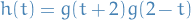
satisfies
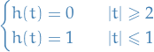
Similarily in the multidimensional case we let
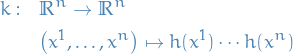
Then,
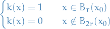
for any  and
and  .
.
Then  and
and  is a function on , i.e. an open neighborhood of .
Let
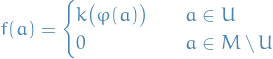
with  . Then .
Can construct functions on entirety of by locally "extending" (i.e. multiply by bump function) already defined functions.
Integration
Integration on manifolds
Motivation
- Want to define integration on manifolds
Need definition to be independent of charts
- Consider chart of
which is the std. Riemann integral
We know that under change of coordinates, the Riemann integral follows

for charts
and , and  denotes the Jacobian of the change of coordinates
Clearly this is not invariant under change of coordinates, unless
which generally is not the case
- Consider chart
 be open

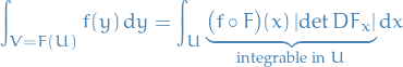
Consider two chart maps on same domain
 and
and  , then instead consider

- Comparing with change of variables, letting
 and
and  , we see that indeed this mathces the std. change of variables excluding the absolute value of
- Comparing with change of variables, letting
- Can we find atlas such that
 for all ?
- If so, then we the absolute value can be "dropped"
Integration
An n-dimensional manifold is orientable if any of the following equivalent properties hold
 is a trivial bundle
 which is nowhere vanishing
- has an atlas
 with
with

in which case we say
 is orientation-preserving.
(This is also kind of a proposition…)
 :
Recall that
:
Recall that  is a trivial bundle if and only if there exists a diffeomorphism
  which is fibrewise linear, so that for all , maps the one-dimensional vector space
  isomorphically to
  .
.
We now show that this is equivalent to there being a nowhere-vanishing section of  . Indeed, given , we defined
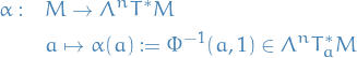
which is a nowhere-vanishing section of . Hence we have one way.
Conversely, if is nowhere-vanishing section of , we define
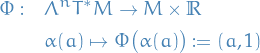
and extending linearly, so that

which gets us the entire 1-dim  , giving us the implication the other way
  .
.
 :
Let
:
Let  be nowhere vanishing, and let be a chart with local coordinates .
Then

for some  which is non-vanishing since is non-vanishing. Without loss of generality we may assume that
  .
.
Let be an overlapping chart, i.e.  , with local coords
  , so
, so

for some 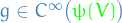 , with (again wlog.)
  .
.
On we then have

where
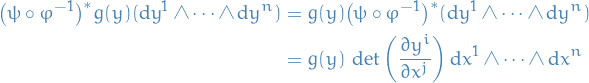
Therefore we have

and since and , then we must have

 :
Let
:
Let
 be an atlas such that

 be a partition of unity subordinate to
  with
with 
Define
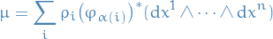
Is
nowhere vanishing?
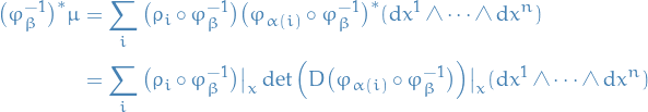
where
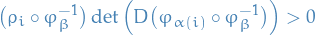
since
 and
and

by assumption.
- Hence is non-vanishing
Show that is always orientable.
Let be orientable.
An orientation on is an equivalence class of nowhere-vanishing n-forms, where two nowwhere-vanishing n-forms 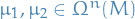 are equivalent if
  with
with  for all such that

Let  be orientable and nowhere vanishing.
Show that given any ,

Consider chart with local frame  , then
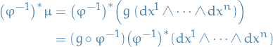
Locally we have


Since is nowhere-vanishing, we know that  . Therefore

gives us

as wanted, which is clearly unique. This holds for arbitrary choice of chart and so on entirety of .

 , i.e. top-form with compact support
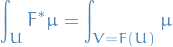
In local frame, there exists  s.t.
s.t.
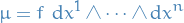
and
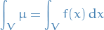
But

so
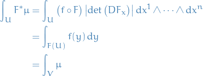
where we have used the fact that
since is orientation-preserving, is orientable and is nowhere-vanishing (and therefore defines an orientation of ).
Let be a n-dimensional oriented manifold (orientable and a choice of orientation).
Then there exists a unique linear map (integration)
such that if is an oriented chart and  , then
LHS is Riemann integral which is of course linear, so we only need to prove that the map is well-defined and unique.
Suppose
 and and
  are two oriented charts. Then

where in
 we simply used Lemma lemma:integral-of-pullback-is-integral-over-image-of-top-form with
  , hence the map is unique.
- Let
 and let be an oriented atlas.
Since
 is compact, there are finitely many
  with
with
Let

- Let
 be a partition of unity subordinate to
  .
.
- Notice:
 since does not have support on
- Notice:
Define
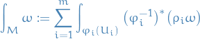
- Need to show that this is independent of choices
- Let
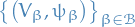 be another oriented atlas
  cover
cover - Let
 and
and  a partition of unity subordinate to
By 1., for all

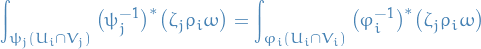
Therefore
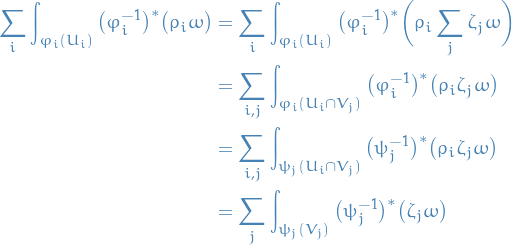
Hence the integral is well-defined.
Stokes Theorem (v1)
 .
.

We follow similar notation as in the proof of integration on manifold. That is
 and
and 
- a partition of unity subordinate to
Then
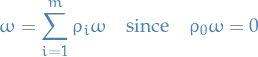
Therefore
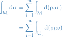
and so the claim is equivalent to claiming

Now,
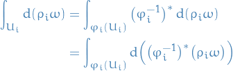
since the exterior derivative commutes with the pull-back.
Observe then that

for  , so that
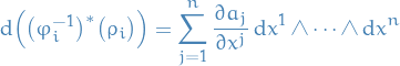
and hence
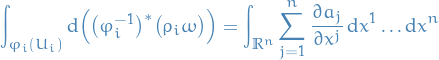
Focus on one such integral (Fubini-Tonelli):
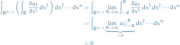
since  has compact support.
Similarily we can repeat this process for all  , which implies that
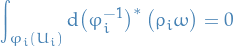
and similariliy for the rest of the terms, concluding our proof.
- Defined integration by summer up contributions weighted by partitions of unity
- Seldom arises the need to do this in order to compute an integral
Most reasonable manifolds (e.g. the sphere) have charts which are valid everywhere except on a subspace of positive codimension, which we recall is defined

for subspace
 .
.
- For subspace of positive codimension, the Riemann integral is vanish
- Thus, we can simply ignore that the chart is not global, safe in the knowledge that the integral will give the correct result!

Let define an orientation. Then ![$[\mu] \in H_{dR}^n(M)$](../../assets/latex/geometry_8e95625be02130765740c9f6624d7b1a7ddcb12e.png) .
.
Integrating,
but if  , then by Stokes' theorem
So
![\begin{equation*}
[\mu] \ne 0
\end{equation*}](../../assets/latex/geometry_9573c21ddffa4b86d699e25016cc674baa594627.png)
Since recall that if ![$[\mu] = [0]$](../../assets/latex/geometry_6d8de9881854b8a47d1341af4c1a4d7ed550839b.png) , then can be written as for some
, then can be written as for some  .
.
Manifold with boundary
An n-dimensional manifold with boundary is a set with a collection  of subsets and maps
  such that

 is a bijection onto an open (in the subspace topology of
  ) subset of
  and
and
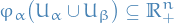
is open for all
.
 is the restriction of maps from neigbhorhood of
  to
to
In short, a manifold with boundary is locally diffeomorphic to . Here we used the notation
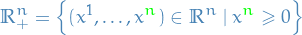
The boundary  of is defined as
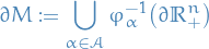
where
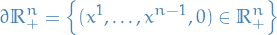
i.e.

Recall that

i.e. the closure of minus the interior of .
Therefore these charts are adapted to and make into an (n - 1)-dimensional submanifold of .
Let
- be a smooth atlas for , a manifold with

- as a submanifold with

If there exists an atlas for , denoted 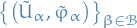 , such that
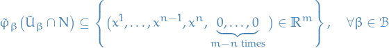
Then we say that is adapted to .
In words, we say a chart is adapted to if  components vanish in the charts.
Definition of adapted charts is just taking a chart and finding a different chart which covers the same subspace, for which we have the above.
Examples

 given by
 ![$M \times [0, 1]$](../../assets/latex/geometry_ff2da6bc074f8a10532d067aa0ade4cf54ae146d.png) is a
is a 
 and
and Differential forms on manifold with boundary
- Differential forms are defined in a similar way
- Locally just restrictions of smooth forms on some open subset of to
- Let
 denote the inclusion
 Can restrict differential forms on
to via the pull-back:

If a manifold with boundary is oriented, then there is an induced orientation on .
- Choose local coordinate systems where is defined by

- Let

On overlapping neighborhoods

On the boundary the Jacobian takes the form
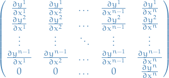
- The lower row is almost filled with zeros as a result of
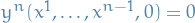 for all
  . This equality holding for all possible
  , implies that
  must be independent of these, hence derivative vanish.
- The lower row is almost filled with zeros as a result of
From def. of manifold with boundary, the transition function maps
 by
by  so that if and
  one must have
From the above jacobian matrix, we have
- Just consider the "standard" way of computing the determinant of a matrix using the "block-expansion" or whatever you want to call it (it's the cofactor expansion, you fool)
Therefore

thus we have transition functions with positive determinant, which we know gives a orientation on
 .
.
- So orientation of induces an orientation on , but which orientation one chooses is a matter of convention.
- For
 this is the choice of "inward" vs. "outward" normal.
 Our choice: if
 defines an orientation on , with
  defining locally, then

is the induced orientation on
- E.g. cylinder, the boundary circles inherit opposite orientations
Generalized Stokes Theorem
Let
- be an n-dimensional manifold with boundary
 have compact support
Then with the induced orientation
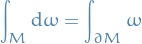
Let
be a partition of unity subordinate to an atlas, then
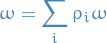
then
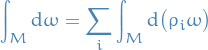
- The sum is finite because is compactly supported
- The sum is finite because
- We have two kinds of charts:
- Those which intersect
- Those who don't
- These do not contribute to the integral over
- This is seen from the proof of the less general case of Stokes' theorem
- These do not contribute to the integral over
- Those which intersect
If the chart does intersect
, we have as in proof of the less general case of Stokes' theorem
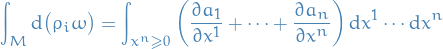
- For all
 expect
  , the integral vanishes because is compactly supported (again look back at the proof for Stokes v1)
 For
 we get
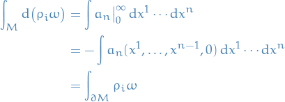
- where we have used the choice of outward normal
- where we have used the choice of outward normal
- Theorem follows by summing the contributions from all charts.
Observe that for the case ![$M = [a, b] \subset \mathbb{R}$](../../assets/latex/geometry_e379c617722dd10d46997daf5e4240c81ab35393.png) , then generalized Stokes theorem says that
, then generalized Stokes theorem says that
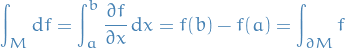
which is just the Fundamental Theorem of Calculus!
Similarily, it agress with Green's theorem, the divergence theorem and, of course the original Stokes' theorem.
Application of Stokes' theorem
Let  be the (closed) unit ball and let
  be a smooth map.
Then has a fixed point.
Suppose there is no fixed point, so

- For each
 , let the ray starting at
  and passing by intersection the boundary sphere at the point
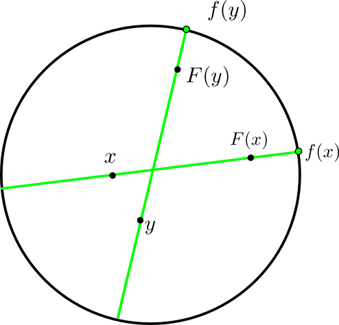
Gives rise to smooth function
 such that
- Clearly
 is orientable and thus
  is also orientable
 Let
 be a nowhere-vanishing (n - 1)-form defining the orientation on
  and normalize it so that
Let
 denote the inclusion so
Then,

where in the equalities follow because:
- Follows from Exercise exercise:pull-back-of-orientation-preserving-diffeo-preserves-integration
- Stokes' theorem

- Since
 , there must exists a fixed point!
 be an
be an  .
.
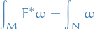
- We have the following sequence of implications
- is diffeo
 is an isomorphism for every and so is its dual
 vanishes at if and only if vanishes at

- And since is homeomorphisms,
 is compact in because is compact in
- Can integrate it
- Let be an oriented atlas atlas for and let
 be a partition of unity subordinate to the open cover .
- Then
 is an oriented atlas of
 defines a covering of since is diffeo
 is a diffeo since composition of diffeos
 is partition of unity subordinate to
Therefore
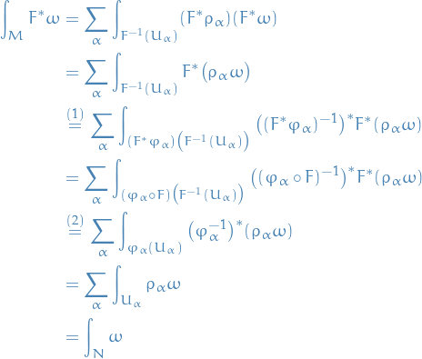
where in
we simply used the "definition" of integration on a manifold, and in  have used the fact that

- Then
Integrations on chains
Notation
![$[0, 1]^k \subset \mathbb{R}^k$](../../assets/latex/geometry_e250261b44719c68af4d332e0feae41a21dc6ed9.png) is the standard unit cube in
is the standard unit cube in  open
open![$c: [0, 1]^k \to U$](../../assets/latex/geometry_bdcb1ea87416a095672ecd530d16ad693d7276f5.png) denotes a singular k-chain
denotes a singular k-chain
k-cubes
Let be open.
A singular k-cube in is a continuous map .
- A singular 0-cube in is, in effect, just a point of
- A singular 1-cube in is parametrized cuvre in
The standard (singular) k-cube is the inclusion map ![$i^k: [0, 1]^k \to \mathbb{R}^k$](../../assets/latex/geometry_1fbe6b35cc98f3c1fd59a3fc05f8458339fdcb60.png) of the standard unit cube.
of the standard unit cube.
A (singular) k-chain in is a formal finite sum of singular k-cubes in with integer coefficients, e.g.

k-chains are then equipped with addition and scalar multiplication by integers.
Boundary of chain
Consider inclusion mapping to the standard k-cube .
For each with  we define two singular (k - 1)-cubes:
![\begin{equation*}
\begin{split}
i_{(j, 0)}^k: \quad & [0, 1]^{k - 1} \to [0, 1]^k \subset \mathbb{R}^k \\
& \big( x^1, \dots, x^{k - 1} \big) \mapsto \big( x^1, \dots, x^{j - 1}, 0, x^j, \dots, x^{k - 1} \big)
\end{split}
\end{equation*}](../../assets/latex/geometry_806379bd57176bfdd0f6a4f6d4dce94d4058eb89.png)
and
![\begin{equation*}
\begin{split}
i_{(j, 1)}^k: \quad & [0, 1]^{k - 1} \to [0, 1]^k \subset \mathbb{R}^k \\
& \big( x^1, \dots, x^{k - 1} \big) \mapsto \big( x^1, \dots, x^{j - 1}, 1, x^j, \dots, x^{k - 1} \big)
\end{split}
\end{equation*}](../../assets/latex/geometry_feee838e37a6af09b2f94937cf0d1a8d27370e34.png)
We refer to these as the  and
and  of
of  , respectively.
Then we define
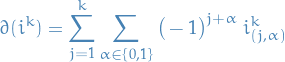
Now, if is a singular k-cube in , we define its  by
by
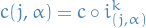
and then define
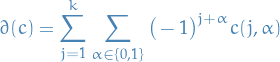
We extend the definition of boundary to k-chains by linearity:
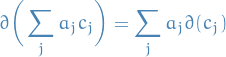
If is a k-chain in , then  , i.e.
Woah! Seems to corresponding heavily with as stated thm:exterior-derivative-squred-is-zero.
Integration
Now let ![$\omega \in \Omega([0, 1])^k$](../../assets/latex/geometry_df69e15472aab95ab5115d21832e043958375063.png) , i.e. is a differential k-form on the unit k-cube
, i.e. is a differential k-form on the unit k-cube ![$[0, 1]^k$](../../assets/latex/geometry_0d1d498fd2d85213e16eb083c21e47e1dc956ec6.png) in . Then
in . Then

In which case we define the integral
![\begin{equation*}
\int_{[0, 1]^k}^{} \omega = \int_{[0, 1]^k}^{} f = \int_{[0, 1]^k}^{} f \big( x^1, \dots, x^k \big) \dd{x^1} \wedge \dots \wedge \dd{x^k}
\end{equation*}](../../assets/latex/geometry_ffdb594dc0940ae544f8fce36b836ddbc141ecbf.png)
If instead  for open , and is a singular k-cube in , we define
![\begin{equation*}
\int_{c}^{} \omega = \int_{[0, 1]^k}^{} c^* \omega
\end{equation*}](../../assets/latex/geometry_a4e99872cbc9fa1828ab331e025c8e74d60d7a28.png)
i.e. integration of a k-form over a singular k-cube is defined by pulling the k-form back to the unit k-cube in and then doing ordinary integration.
By linearity, for a singular k-chain  ,
,
Cartan calculus
Notation
 denotes the vector space of degree-k derivatives
Derivation
A derivation is a linear map

for some algebras and , which additionally satisfies the Leibniz rule, that is:

where  and
and  denotes the products in the algebras and respectively.
In particular, if  and
and  , then

Moreover, we define to be the vector space of degree-k derivatives.
One can also show that if  and
and  , then

Example: derivative on algebra of continuous functions
We have the algebra  , for any , we have

which satisfies
Example: Lie-algebra
Let  for some K-vectorspace , then we define the map
defined by
![\begin{equation*}
[\varphi, \psi] = \varphi \circ \psi - \psi \circ \varphi
\end{equation*}](../../assets/latex/geometry_0a928f8b5fbeeb1ef22e4bda691a9babe8b5d4fa.png)
then  forms an algebra, which is an example of a Lie-algebra!
In fact, the definition of a Lie-algebra is because of some other property, but this is an example of a Lie-algebra.
Stuff
Let  and let
  be the local flow of , i.e. for all
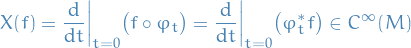
Moreover, let  .
.
We define the Lie derivative of along  by
by
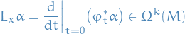
Then

For all , we have  and
and

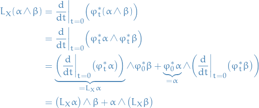
Let .
The contraction with is a linear map
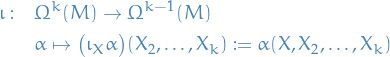
For , we have  .
.
Moreover,


For all  and
and  (the Grassman algebra),
 where
where 
 where
where 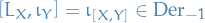
 where
where 
Temp


is an ideal, and

is abelian.

since

because
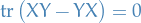
And

Q & A
DONE Tangent spaces and their basis
- Note taken on
See my note at the end of the question
When we're talking about a tangent space , we say the space is defined by the basis of all the differential operators , i.e.
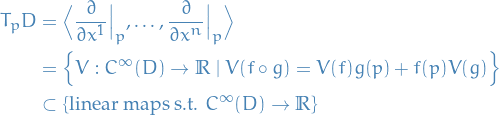
Now, these , are they arbitrary? Or are they dependent on the fact that we can project them onto Euclidean space in some way, i.e. reparametrise some arbitrary basis  to
to  .
.
I believe so. In fact, the notation we're using here is that , hence we're already assuming the domain to actually be in , i.e. there always exists a reparametrisation to "normal" Euclidean coordinates.
DONE Is the tangent space at each point an intrinsic property or does it depend on the embedding space?
- Note taken on
It turns out, the tangent space can be described without an embedding space!