Variational Calculus
Table of Contents
Sources
- Most of these notes comes from the Variational Calculus taught by Prof. José Figueroa O'Farrill, University of Edinburgh
Overview
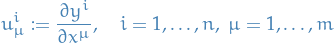
Notation
 denotes the space of possible paths (i.e.
  curves) between points
  and
and 
Introduction
Precise analytical techniques to answer:
- Shortest path between two given points on a surface
- Curve between two given points in the place that yields a surface of revolution of minimum area when revolved around a given axis
- Curve along which a bead will slide (under the effect of gravity) in the shortest time
Underpins much of modern mathematical physics, via Hamilton's principle of least action
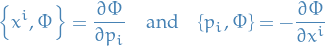
Consider "standard" directional derivative of  , with
  , at
, at  along some vector
  :
:
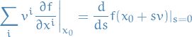
where is a critical point of  , i.e.
(since we know that  form a basis in
  , so by lin. indep. we have the above!)
Stuff
Let ![$f: [0, 1] \to \mathbb{R}^n$](../../assets/latex/variational_calculus_d3d2ff9a96e78f64c0ee8b8098a856d71b2f4fd8.png) be a continuous function which satisfies
be a continuous function which satisfies
for all ![$h \in C^{\infty}\Big([0, 1], \mathbb{R}^n\Big)$](../../assets/latex/variational_calculus_b1c6c1d30a3cbd38cb80c74ef5f3f7c55f8109ae.png) with
with
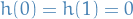
Then  .
.
Observe that if we only consider  , then we can simply genearlize to arbitrary
  since integration is a linear operation.
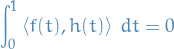
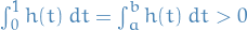
Let ![$f \in C([0, 1])$](../../assets/latex/variational_calculus_795511f38a674f2eca972b1e89f37e957086b05e.png) which obeys
which obeys
![\begin{equation*}
\int_{0}^{1} f(t) h(t) \ dt = 0, \quad \forall h \in C^{\infty}([0, 1]), h(0) = h(1) = 0
\end{equation*}](../../assets/latex/variational_calculus_e0c2b4dc4a4446fa8cd714fab12dc08fa3b150e6.png)
Assume, for the sake of contradiction, that  , i.e.
![\begin{equation*}
\exists t_0 \in [0, 1] : f(t_0) \ne 0
\end{equation*}](../../assets/latex/variational_calculus_92ecc6e7731feb6bc2cc1a5379e2ae02babb0be0.png)
Let, w.l.o.g.,  .
.
Since is continuous, there is some interval  such that
  and some
  such that
![\begin{equation*}
f(t) > c, \quad \forall t \in [0, 1]
\end{equation*}](../../assets/latex/variational_calculus_6e1a0080a7ecbbf476287ad11c79c3a9cd61f175.png)
Suppose for the moment that there exists some ![$h \in C^{\infty}([0, 1])$](../../assets/latex/variational_calculus_47d6afce147f878df38ac46eb3ab58898a523db5.png) such that
such that
 for all
  outside
Then observe that
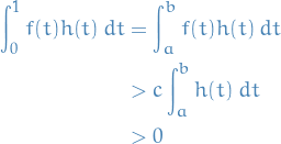
This is clearly a contradiction with our initial assumption, hence  such that
  . Hence, by continuity,
![\begin{equation*}
f(t) = 0, \quad \forall t \in [0, 1]
\end{equation*}](../../assets/latex/variational_calculus_4e4705bde280555067774281e86c75a20e622823.png)
Now we just prove that there exists such a function  which satisfies the properties we described earlier.
Let
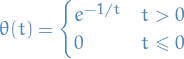
which is a smooth function. Then let

which is a smooth function, since it's a product of smooth functions.
To make this vanish outside of , we have
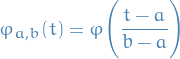
This function is clearly always positive, hence,
Hence, letting  we get a function used in the proof above!
This concludes our proof of Fundamental Lemma of the Calculus of Variations
General variations
Suppose we want te shortest path in  between and a curve
  on .
on .
We assume that  with
with  differentiable, such that
  .
.
Then observe that  , then

Then
![\begin{equation*}
\begin{split}
\frac{d}{ds} S[x_s] &= \frac{d}{ds} \bigg|_{s = 0} \int_{0}^{1} \norm{\dot{x}_s} \ dt \\
&= \int_{0}^{1} \left\langle \dot{\xi}, \frac{\dot{x}}{\norm{\dot{x}}} \right\rangle \ dt \\
&= \int_{0}^{1} \Bigg( \frac{d}{dt} \left\langle \xi, \frac{\dot{x}}{\norm{\dot{x}}} \right\rangle - \left\langle \varepsilon, \frac{d}{dt} \bigg( \frac{\dot{x}}{\norm{\dot{x}}} \bigg) \right\rangle \Bigg) \ dt \\
&= \left\langle \varepsilon(1), \frac{\dot{x}(1)}{\norm{\dot{x}(1)}} \right\rangle - \underbrace{\left\langle \varepsilon(0), \frac{\dot{x}(0)}{\norm{\dot{x}(0)}} \right\rangle}_{= 0} - \frac{0}{1} \left\langle \varepsilon, \frac{d}{dt} \bigg( \frac{\dot{x}}{\norm{\dot{x}}} \bigg) \ dt \right\rangle \\
&= \left\langle \varepsilon(1), \frac{\dot{x}(1)}{\norm{\dot{x}(1)}} \right\rangle - \frac{0}{1} \left\langle \varepsilon, \frac{d}{dt} \bigg( \frac{\dot{x}}{\norm{\dot{x}}} \bigg) \ dt \right\rangle
\end{split}
\end{equation*}](../../assets/latex/variational_calculus_62a7e95257987602bb41eb7c56505353fc431de0.png)
where we've used the fact that
We cannot just drop the endpoint-terms anymore, since these are now not necessarily vanishing, as we had in the previous case.
Then, by our earlier assumption, we have
which implies that
Hence,
must hold for all ![$\varepsilon: [0, 1] \to \mathbb{R}^2$](../../assets/latex/variational_calculus_e526d89ca91142c7e7c1d3593fa54343088c0d71.png) and
and  and
and 
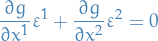
In particular,  , then
and
i.e.  is normal to at the point where it intersects with .
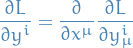
Euler-Lagrange equations
Notation
 or
or  denotes the Lagrangian
Endpoint-fixed variations
Let be the space of curves ![$x: [0, 1] \to \mathbb{R}^n$](../../assets/latex/variational_calculus_4c004d0dd181c4042e1bb961df5af02834eb5298.png) with
with

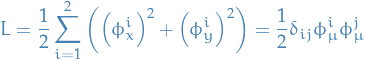
The Lagrangian is defined
where  and
and  . Let be "sufficiently" differentiable (usually taken to be smooth in applications).
Then the function  , called the action, is defined
![\begin{equation*}
I[x] = \int_{0}^{1} L \Big( x(t), \dot{x}(t), t \Big) \ dt
\end{equation*}](../../assets/latex/variational_calculus_405689cc14d60b17f3786d96cf09a2f1ab843d37.png)
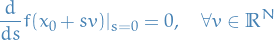
A path  is a critical point for the action if, for all endpoint-fixed variations
  , we have
![\begin{equation*}
\frac{d}{ds} I [x + s \varepsilon] \Big|_{s = 0} = 0
\end{equation*}](../../assets/latex/variational_calculus_633393a3128b9a2c82928d3d5f2d65025baf987b.png)
Bringing the differentiation into to the integral, we have
![\begin{equation*}
\begin{split}
\frac{d}{ds} I[x + s \varepsilon] &= \int_{0}^{1} \frac{d}{ds} \Big|_{s = 0} L \Big( x + s \varepsilon, \frac{d}{dt}(x + s \varepsilon), t \Big) \ dt \\
&= \int_{0}^{1} \frac{d}{ds} \Big|_{s = 0} L \Big( x + s \varepsilon, \dot{x} + s \dot{\varepsilon}, t \Big) \ dt \\
&= \int_{0}^{1} \bigg( \sum_{i=1}^{n} \frac{\partial L}{\partial x^i} \varepsilon^i + \sum_{i=1}^{n} \frac{\partial L}{\partial \dot{x}^i} \dot{\varepsilon}^i \bigg) \ dt \\
&= \int_{0}^{1} \sum_{i=1}^{n} \bigg( \frac{\partial L}{\partial x^i} - \frac{d}{dt} \frac{\partial L}{\partial \dot{x}^i} \bigg) \varepsilon^i \ dt
\end{split}
\end{equation*}](../../assets/latex/variational_calculus_a3251b09dcea3d9b1aa697c90c06ba4828210271.png)
Properties
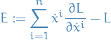
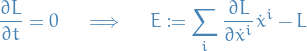
If
 , then the "energy" given by
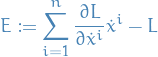
is constant along extremals of the Lagrangian. Then observe that
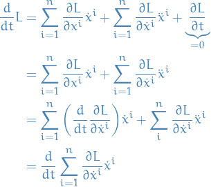
where we've used the fact that
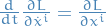 in the thrid equality.
Thus,
in the thrid equality.
Thus,
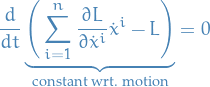
and,

Hence,

i.e time invariance! This is an instance of Noether's Theorem.
If , so that the lagrangian does not depend explicitly on , then the energy
is constant.
This is known as the Beltrami's idenity.
Euler-Lagrange
Let be the space of curves with
Let
where and , be sufficiently differentiable (typically smooth in applications) and let us consider the function defined by
![\begin{equation*}
I[x] = \int_{0}^{1} L \big( x(t), \dot{x}(t), t \big) \ dt
\end{equation*}](../../assets/latex/variational_calculus_081b2b6f8ab94dd38a6ebed66b324fc303063efb.png)
Then he extremals must satisfy the Euler-Lagrange equations:
Newtonian mechanics
Notation
worldlines refer to the trajectory of a particle:

with

Galilean relativity
- Affine transformations (don't assume a basis)
- Relativity group: group of transformations on the universe preserving whichever structure we've endowed the universe with
The subgroup of affine transformations of  which leave invariant the time interval between events and the distance between simultaneous events is called the Galilean group.
That is, the Galilean group consists of affine transformations of the form

These transformations can be written uniquely as a composition of three elementary galilean transformations:
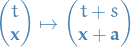
translations in space and time:
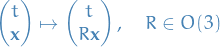
orthogonal transformations in space:
and galilean boosts:
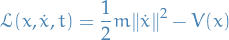
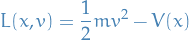
Observe that if choose the action
![\begin{equation*}
I[x] = \int_{0}^{1} \bigg( \frac{1}{2} m \norm{\dot{x}}^2 - V(x) \bigg) \ dt
\end{equation*}](../../assets/latex/variational_calculus_c8540466e49d2efb40dbe1bc11adf27237c7c85a.png)
which has Lagrangian
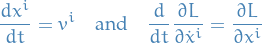
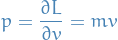
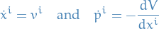
then we observe that the minimizing path should satisfy
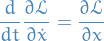
which is
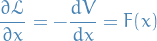
where  denotes the force. Further,

which is the momentum! Then,
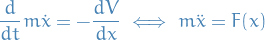
Hence we're left with Newton's 2nd law.
Noether's Theorem
Notation
 of
of  functions called one-parameter subgroup of diffeomorphisms , which are differentiable wrt.
 and
and  are defined by
and


Stuff
We've seen the following continuous symmetries this far:
Momentum is conserved:
Energy is conserved:
We say that  is a symmetry of the Lagrangian if

where

- is a diffeomorphism
Equivalently, one says that is invariant under .
Let of functions, defined for all  and depending differentiably on .
Moreover, let this family satisfies the following properties:
 for all
 for all
Then the family  is called a one-parameter subgroup of diffeomorphisms on
  .
.
Let ![$I[x] = \int_{0}^{1} L(x, \dot{x}, t) \ dt$](../../assets/latex/variational_calculus_df566f10058cb409490a4cb7e6c1d8456e18faac.png) be an action for curves , and let be invariant under a one-parameter group of diffeomorphisms .
be an action for curves , and let be invariant under a one-parameter group of diffeomorphisms .
Then the Noether charge  , defined by
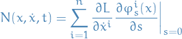
is conserved; that is,  along physical trajectories.
Consider functions which are defined by Lagrangians  and such that they are invariant under one-parameter family of diffeomorphisms of
  such that
This means, in particular, that
where
Then the Noether charge
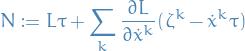
is conserved along extremals; that is, along curves which obey the Euler-Lagrange equation.
Hamilton's canonical formalism
Notation
Considering
![\begin{equation*}
I[x] = \int_{0}^{1} L(x, \dot{x}, t) \ dt
\end{equation*}](../../assets/latex/variational_calculus_a2813c71b2588557d1eabe19c2329053edc7a8d2.png)
for
curves
- Differentiable function

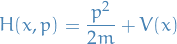
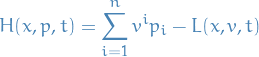
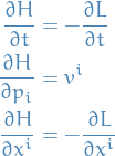
 denotes the Hamiltonian
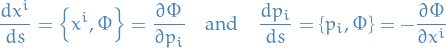
Canonical form of Euler-Lagrange equation
Can convert E-L into equivalent first-order ODE:
is equivalent to system
for the variables
 .
.
Consider
Then letting
the above system becomes
Hamiltonian becomes
which has the property
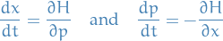
known as Hamilton's equations.
Observe that
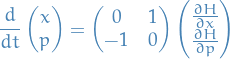
where the coefficient matrix, let's call it
 , can be thought of as a bilinear form on , which defines a symplectic structure.
- In general case, existence of solution set to the equations is guaranteed by the implicit function theorem in the case where the Hessian
 is invertible
- is then said to be regular (or non-degenerate)
General case:
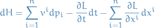
Hamiltonian
Total derivative of
(or as we recognize, the exterior derivative of a continuous function)
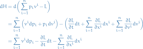
where we have used that
 .
.
Give us
First-order version of Euler-Lagrange equations in canonical (or hamiltonian) form:
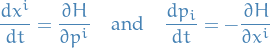
which we call Hamilton's equations.
In general, the Hamiltonian  is given by
Taking the total derivative, we're left with
where we've used .
This gives us
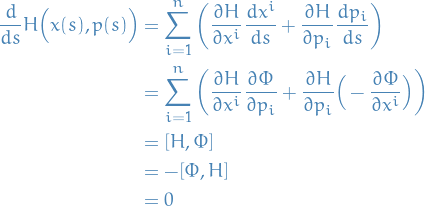
Conserved quantity using Poisson brackets
Consider energy conserved, i.e.  , and a differentiable function :
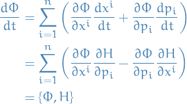
where we have introduced the Poisson bracket
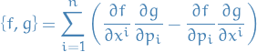
for any two differentiable functions  of
of  .
.
Hence
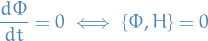
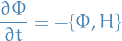
If  depend explicity on , then the same calculation as above would show that
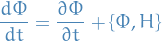
In this case could still be conserved if
Given two conserved quantities  and
and  , i.e. Poisson-commute with the hamiltonian .
Then we can generate new conserved quantities from old using the Jacobi identity:

Therefore  is a conserved quantity.
Can we associate some * to an conserved charge?
Consider a conserved quantity which satisfy

Then
defines a vector field on the phase space  which we may integrate to find through every point a solution to the differential equation
Then, by existence and uniqueness of solutions to IVPs on some open interval  as given above, gives us the unique solutions
  and
and  for some initial values
  and
and  .
.
Therefore,
Thus we have a continuous symmetry of Hamilton's equations, which takes solutions to solutions.
That is, these solutions  which are in some sense generated from and contain symmetries!
E.g. solution to the system of ODEs above could for example be a linear combination of  and
and  , in which case we would then understand that "symmetry" generated by is rotational symmetry.
The caveat is that this may not actually extend to a one-parameter family of diffeomorphisms, as we used earlier in Noether's theorem as the invariant functions or symmetries.
Example:
Lagrangian:
![\begin{equation*}
L[x^{\mu}, \dot{x}^{\mu}] = \sqrt{- \eta_{\mu \nu} \dot{x}^{\mu} \dot{x}_{\nu}
\end{equation*}](../../assets/latex/variational_calculus_3cca97173bbd30075480959c48d713a3a788a0c1.png)
Exists
TODO Integrability
A set of functions which Poisson-commute among themselves are said to be in involution.
Liouville's theorem says that if a hamiltonian  on admits independent conserved quantities in involution, then there is a canonical transformation to so called action / angle variables
  such that Hamilton's equations imply that

Such a system is said to be integrable.
Constrained problems
Isoperimetric problems
Notation
Typically we talk about the constrained optimization problem:
![\begin{equation*}
\begin{split}
J[y] &= \int_{0}^{1} L(y, y', x) \dd{x} \\
\text{subject to} \quad I[y] &= \int_{0}^{1} K(y, y', x) \dd{x} = 0 \\
& y(0) = y_0, \quad y(1) = y_1
\end{split}
\end{equation*}](../../assets/latex/variational_calculus_f7e15f5e02753d07332864e2ae757a372098da2b.png)
for
![$y: [0, 1] \to \mathbb{R}^n$](../../assets/latex/variational_calculus_6d3466088c0db0a754bf0b0b0ad661573242983a.png) .
.
Stuff
- Extremise a functional subject to a functional constraint
Consider a closed loop enclosing some area  .
.
The Dido's problem or (original) isoperimetric problem is the problem of maximizing the area of while keeping the length of constant.
Consider  for
for ![$t \in [0, 1]$](../../assets/latex/variational_calculus_64ff94a722f22cff3ff97e2f423a713eb1e42c4e.png) with initial conditions
with initial conditions
Using Green's theorem, we have

and length
The problem is then that we want to extremise ![$I [x, y] = \frac{1}{2} \big( x \dot{y} - y \dot{x} \big)$](../../assets/latex/variational_calculus_f9475841f2d60bb7a73526ab0fcfce9dada64669.png) wrt. the constraint
wrt. the constraint ![$J[ x, y] = \ell$](../../assets/latex/variational_calculus_12e401bb3847cc1e1fbd16334c4c45789070165f.png) .
.
More generally, given functions for
![\begin{equation*}
\begin{split}
y: \quad & [0, 1] \to \mathbb{R}^n \\
& x \mapsto y(x)
\end{split}
\end{equation*}](../../assets/latex/variational_calculus_14d529b5bf557b65d7c592eda91ab7ac627fab41.png)
being endpoint fixed, e.g.  and
and  for some
  .
.
Given the functionals
![\begin{equation*}
\begin{split}
I[y] &= \int_{0}^{1} L(y, y', x) \dd{x} \\
J[y] &= \int_{0}^{1} K(y, y', x) \dd{x}
\end{split}
\end{equation*}](../../assets/latex/variational_calculus_d7320916d6cd62474994e859d17a57803ceef358.png)
we want to extremise  subject to
  .
.
Let  and let
  be an extremum of subject to
  .
.
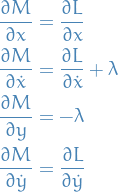
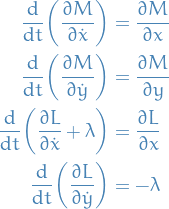
If  (i.e. is not a critical point), then
  (called a Lagrange multiplier) s.t.
  is a critical point of the function
  defined by
Supose  is an extremal of in the space of with
 ![$J[y] = 0$](../../assets/latex/variational_calculus_09fd96413c1791ad8370554cd5654a06a1cbe6d2.png) . Then
. Then
![\begin{equation*}
\frac{d}{ds}\bigg|_{s = 0} I[Y_s] = 0 \quad \text{subject to} \quad J[Y_s] = 0
\end{equation*}](../../assets/latex/variational_calculus_f54cb42cdaa13dd7e430936cb76961c2a3385ec0.png)
for small , where  .
.
This might constrain
and prevent use of the Fundamental Lemma of Calculus of Variations.
Idea:
- Consider
 and
and  for all
  near
near  , defined
  .
. - Then express one of the variations as the other, allowing us to eliminate one.
Let  be defined
![\begin{equation*}
\begin{split}
f(r, s) &:= I[Y_{r,s}] \\
g(r, s) &:= J[Y_{r, s}]
\end{split}
\end{equation*}](../../assets/latex/variational_calculus_43f11f3643bd9494ebf4f6887757ed84e27ad8ab.png)
Assume now that  and
and  .
.
If we specifically consider (wlog)  , then IFT implies that
for "small" . Therefore,
is a
Let
![\begin{equation*}
\begin{split}
J[y] &= \int_{0}^{1} L(y, y', x) \dd{x} \\
I[y] &= \int_{0}^{1} K(y, y', x) \dd{x}
\end{split}
\end{equation*}](../../assets/latex/variational_calculus_272613f68955b4ed87aa680ca4e04e0a862fb79f.png)
be functionals of functions ![$y: [0, 1] \to \mathbb{R}$](../../assets/latex/variational_calculus_18e1a26d685fe12448d54b5d7572a2e7d8a5b5c6.png) subject to BCs
subject to BCs

Suppose that  is an extremal of subject to the isoperimetric constraint
 ![$I[y] = 0$](../../assets/latex/variational_calculus_7f8f190a51567df2b008a3ef690d93d8c132c896.png) . Then if is not an extremal of
. Then if is not an extremal of ![$I[y]$](../../assets/latex/variational_calculus_d31a379e90855b527882bb108eacec5327d24349.png) , there is a constant
, there is a constant  so that is an extremal of
 ![$J[y] - \lambda I [y]$](../../assets/latex/variational_calculus_7427fa969ac98b1dec0c6a0e11d68a3fd8813360.png) . That is,
. That is,
![\begin{equation*}
\exists \lambda \in \mathbb{R}: \quad J[y] - \lambda I [y] = \max_{y' \in C^1} J[y'] - \lambda I [y']
\end{equation*}](../../assets/latex/variational_calculus_b0f50e04b3632afe2e846c248334f0e4872496c0.png)
Method of Lagrange multipliers for functionals
Suppose that we wish to extremise a functional
for .
Then the method consists of the following steps:
- Ensure that has no extremals satisfying .
Solve EL-equation for

which is second-order ODE for
.
- Fix constants of integration from the BCs
- Fix the value of
 using .
Classical isoperimetric problem
The catenary
Notation
 denotes height as a function of arclength
Catenary
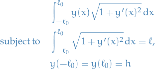
- Uniform chain og length
 hangs under its own weight from two poles of height
  a distance
  apart
apart Potential energy is given by
 , which we can parametrize
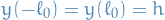
![\begin{equation*}
y(x) = H \Big( s(x) \Big), \quad x \in [- \ell_0, \ell_0]
\end{equation*}](../../assets/latex/variational_calculus_fc93a7edc05ad3f51067016241462ec395c3a81a.png)
giving us
- Observation:
- All extremals of arclength are straight lines
- Extremal to constrained problem has non-zero gradient of the constraint
- → straight lines are not the solutions
Consider lagrangian
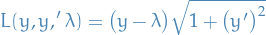
Using Beltrami's identity:
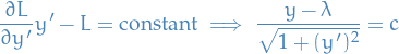
rewritten to
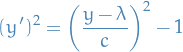
which, given the BCs
 we get the solution
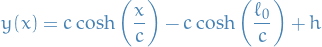
which follows from taking the derivative of both sides and then solving.
Impose the isoperimetric condition:
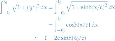
Introducing
 , we find the following transcendental equation

for which
 is the trivial solution
 small, together with the condition
  ensures that
But for
 the exponential term dominates

by continuity.
Holonomic and nonholonomic constraints
- Constraints are simply functions, i.e.
 for some
- Instead of functionals
 as we saw for isoperimetric problems
- Instead of functionals
We say a constraint is scleronomic if the constraint does not depend explicitly on , and rheonomic if it does.
We say a constraint is holonomic if it does not depend explicitly on  , and nonholonomic if it does.
In the case where nonholonomic constraints are at most linear in , then we say that the constraints are pfaffian constraints.
Typical usecases
- Finding geodesics on a surface as defined as the zero locus of a function, which are scleronomic and holonomic.
- Reducing higher-order lagrangians to first-order lagriangians
 can be replaced by
which are scleronomic and nonholonomic.
- Mechanical problems: e.g. "rolling without sliding", which are typically nonholonomic
Holonomic constraints
![\begin{equation*}
\begin{split}
J[x] &= \int_{0}^{1} L(x, \dot{x}, t) \dd{t} \\
\text{subject to} \quad g(x, t) &= 0
\end{split}
\end{equation*}](../../assets/latex/variational_calculus_924e789566074a2e58a8290a35971c6b7fffb7bf.png)
 for all
 ![$\lambda: [0, 1] \to \mathbb{R}$](../../assets/latex/variational_calculus_4644f6d63e5ceb972a6993d51ff0c5d43e905a21.png) such that
such that 
 is the gradient wrt.
  for all
  , NOT .
Let ![$y: [0, 1] \times (- \delta, \delta) \longrightarrow \mathbb{R}^n$](../../assets/latex/variational_calculus_c43bca487b63ecb3d945bad5838cb5789831e2cf.png) be admissible variation of
be admissible variation of  .
.
Then the constraint requires
Let
Then the contraint above implies that
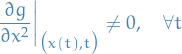
i.e. if  then is tangent to the implicitly defined surface
  .
.
Consider  , then the above gives us
We therefore suppose that
The implicit function then implies that we can solve  for one component. Then the above gives us
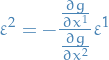
i.e.  is arbitrary and
  is fully determined by in this "small" neighborhood
  .
.
Then
![\begin{equation*}
\begin{split}
\dv{s}\bigg|_{s = 0} I[y] &= \int_{0}^{1} \bigg( \frac{\partial L}{\partial x^i} \varepsilon^i + \frac{\partial L}{\partial \dot{x}^i} \dot{\varepsilon}^i \bigg) \dd{t} \\
&= \int_{0}^{1} \bigg( \frac{\partial L}{\partial x^i} - \dv{t} \frac{\partial L}{\partial \dot{x}^i} \bigg) \varepsilon^i \dd{t} \\
&= \int_{0}^{1} \bigg[ \bigg( \frac{\partial L}{\partial x^1} - \dv{t} \frac{\partial L}{\partial \dot{x}^i} \bigg) \varepsilon^1 - \lambda(t) \underbrace{\frac{\partial g}{\partial x^2} \varepsilon^2}_{- \frac{\partial g}{\partial x^1} \varepsilon^1} \bigg] \dd{t} \\
&= \int_{0}^{1} \bigg( \frac{\partial L}{\partial x^1} - \dv{t} \frac{\partial L}{\partial \dot{x}^1} - \lambda \frac{\partial g}{\partial x^1} \bigg) \varepsilon^1 \dd{t}
\end{split}
\end{equation*}](../../assets/latex/variational_calculus_38c1cecd18e131fe26c222c99412d225912c3f9c.png)
Since is arbitrary, FTCV implies that
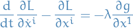
Which is jus the E-L equation for a lagrangian given by

Above we use the implicit function theorem to prove the existence of such extremals, but one can actually prove this using something called "smooth partion of unity".
In that case we will basically do the above for a bunch of different neighborhoods, and the sum them together to give us (apparently) the same answer!
Nonholonomic constraints
Examples
(Non-holonomic) Higher order lagrangians
can be replaced by
which are scleronomic and nonholonomic.
So we consider the Lagriangian

Then
So the E-L equations gives us
which gives us
![\begin{equation*}
\begin{split}
- \dv{}{t} \bigg( \pdv{L}{\dot{x}} \bigg) + \dv[2]{}{t} \bigg( \pdv{L}{\dot{y}} \bigg) + \pdv{L}{x} &= 0 \\
\iff \quad \dv[2]{}{t} \bigg( \pdv{L}{\ddot{x}} \bigg) - \dv{}{t} \bigg( \pdv{L}{\dot{x}} \bigg) + \pdv{L}{x} &= 0
\end{split}
\end{equation*}](../../assets/latex/variational_calculus_807b62ce871bb9fffd005dbcc2ff064069caa02e.png)
where we've used
Variational PDEs
Notation
 be a function on the set
 Lagrangian over a surface
 with corresponding action
![\begin{equation*}
S[y] = \int_D L \big( y, y_u, y_v, u, v \big) \dd{u} \dd{v}
\end{equation*}](../../assets/latex/variational_calculus_f738db80d29dbc145476543789a4e1fe942c9aa1.png)
where
 and
and  denote collectively the
  partial derivatives
  and
and  for
for 
BCs are given by

where
 is given
Variations are
functions  such that

Stuff
Then
![\begin{equation*}
\begin{split}
\dv{}{s}\bigg|_{s = 0} S[y + s \varepsilon] &= \int_{D}^{} \dv{}{s}\bigg|_{s = 0} L \big( y + s \varepsilon, y_u + s \varepsilon_u, y_v + s \varepsilon_v, u, v \big) \dd{u} \dd{v} \\
&= \int_D \bigg( \frac{\partial L}{\partial y^i} \varepsilon^i + \frac{\partial L}{\partial y_u^i} \varepsilon_u^i + \frac{\partial L}{\partial y_v^i} \varepsilon_v^i \bigg) \dd{u} \dd{v} \\
&= \int_D \bigg( \pdv{L}{y^i} - \pdv{}{u} \pdv{L}{y_u^i} - \pdv{}{v} \pdv{L}{y_v^i} \bigg) \varepsilon^i \dd{u} \dd{v} \\
& \quad + \int_D \bigg[ \pdv{}{u} \bigg( \pdv{L}{y_u^i} \varepsilon^i \bigg) + \pdv{}{v} \bigg( \pdv{L}{y_v^i} \varepsilon^i \bigg) \bigg] \dd{u} \dd{v}
\end{split}
\end{equation*}](../../assets/latex/variational_calculus_38c2f450739f944d10926d5022ba830e96ae0670.png)
where we've used integration by parts in the last equality.
The Divergence (or rather, Stokes') theorem allows us to rewrite the last integral as
![\begin{equation*}
\int_{D}^{} \bigg[ \pdv{}{u} \bigg( \pdv{L}{y_u^i} \varepsilon^i \bigg) + \pdv{}{v} \bigg( \pdv{L}{y_v^i} \varepsilon^i \bigg) \bigg] \dd{u} \dd{v} = \int_{\partial D}^{} \bigg( \pdv{L}{y_u^i} N^{u} + \pdv{L}{y_v^i} N^{v} \bigg) \varepsilon^i \dd{\ell}
\end{equation*}](../../assets/latex/variational_calculus_aef6ce5b0a95fb41769490771330cd0768fe40fd.png)
where is the arclength. And since  this vanishes.
Generalisation of the FLCV the first integral term must vanish and so we get
We can generalise this to more than just 2D!
Multidimensional Euler-Lagrange equations
Let
 be a bounded region with (piecewise) smooth boundary.
 denote the coordinates for
  be the Lagrangian for maps
  where
where  denotes collectively the
  partial derivatives
Then the general Euler-Lagrange equations are given by
using Einstein summation.
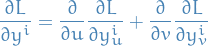
Notice that we are treating  as a function of the x's and differentiate wrt.
  keeping all other x's fixed!
(This is really Stokes' theorem)
Let
- be bounded open set with (piecewise) smooth boundary

 be a smooth vector field defined on
- be the unit outward-pointing normal of
Then,
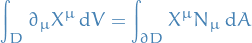
(using Einstein summation) where  is the volume element in
  and
and  is the area element in and
  denotes the Euclidean inner product in .
Let
- be bounded open with (piecewise) smooth boundary
 be a continuous function which obeys
![\begin{equation*}
\int_D \left\langle f(x), h(x) \right\rangle \dd[m]{x} = 0
\end{equation*}](../../assets/latex/variational_calculus_56e01ab924ff3d17db5fd92bd9d2fe8effe3b415.png)
for all
 functions
  vanishing on .
Then .
Noether's theorem for multidimesional Lagrangians
Notation
Lagrangian
![\begin{equation*}
S[u] = \int_D L \big( u, \nabla u, x \big) \dd[m]{x}
\end{equation*}](../../assets/latex/variational_calculus_81473411efe43402ea26d05249812ea39e03e31a.png)
where
Use the notation

Conserved now refers to "divergenceless", that is,
is a conserved quantity if

where we're using Einstein summation.
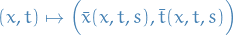
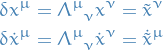
 for denotes a one-parameter group of diffeomorphisms
 is defined
Stuff
We say it's a conserved "current" because
![\begin{equation*}
\pdv{}{x^{\mu}} J^{\mu} = 0 \implies \int_{\partial D} \left\langle N, J \right\rangle \dd[n - 1]{x} = \int_D \underbrace{\text{div} \ J}_{= 0} \dd[n]{x} =\text{constant}
\end{equation*}](../../assets/latex/variational_calculus_bb0defde5ef255cb4d482b319974c9764c8f2978.png)
where
denotes the normal to the boundary
Consider
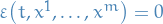
And let
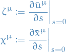
such that
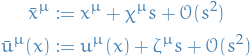
We suppose that the action is invariant, so that the Lagrangian obeys
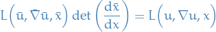
or equivalently, one can (usually more easily) check that the following is true

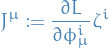
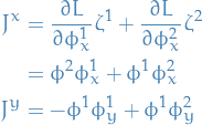
The Noether current is then given by
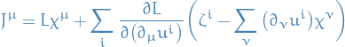
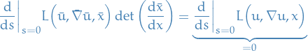
since the RHS is independent of . The LHS on the other hand is given by

where 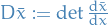 .
.
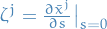
Now we observe the following:

and
![\begin{alignat*}{2}
\pdv[2]{\bar{u}^i}{s}{u^j} \bigg|_{s = 0} &= \pdv{\zeta^i}{u^j} \qquad \pdv[2]{\bar{x}^{\mu}}{s}{x^{\mu}} \bigg|_{s = 0} &= \pdv{\chi^{\mu}}{x^{\nu}} \\
\pdv[2]{\bar{u}^i}{s}{x^{\mu}} \bigg|_{s = 0} &= \pdv{\zeta^i}{x^{\mu}} \qquad \pdv[2]{\bar{x}^{\mu}}{s}{u^i} \bigg|_{s = 0} &= \pdv{\chi^{\mu}}{u^{i}}
\end{alignat*}](../../assets/latex/variational_calculus_5221600b289cd65d26ffdd144b32e551a71f66bf.png)
where we've simply taking the derivatives of the Taylor expansions. Hence, we are left with

Now we need to evaluate  and it's derivative wrt. . First we notice that

We now compute  . We first have
![\begin{equation*}
\begin{split}
\pdv{}{s} \dv{\bar{x}^{\mu}}{x^{\nu}} \bigg|_{s = 0} &= \pdv[2]{\bar{x}^{\mu}}{s}{x^{\nu}} \bigg|_{s = 0} + \sum_{i}^{} \pdv[2]{\bar{x}^{\mu}}{s}{u^i}\bigg|_{s= 0} \pdv{u^i}{x^{\nu}} \\
&= \pdv{\chi^{\mu}}{x^{\nu}} + \sum_{i}^{} \pdv{\chi^{\mu}}{u^i} \pdv{u^i}{x^{\nu}} \\
&= \dv{\chi^{\mu}}{x^{\nu}}
\end{split}
\end{equation*}](../../assets/latex/variational_calculus_3baa417451b11709b3dc31cdd8722e1980279b02.png)
Finally using the fact that if a we have some matrix  given by

we have
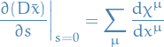
Finally we need to compute  , which one will find to be
AND I NEED TO PRACTICE FOR MY EXAM INSTEAD OF DOING THIS. General ideas are the above, and then just find an expression for the missing part. Then, you do some nice manipulation, botain an expression which vanish due to the EL equations being satisfied by the non-transformed  , and you end up with the Noether's current for the multi-dimensional case.
Examples
Minimal surface
Let  be a twice differentiable function.
The grahp  defines a surface
  . The area of this surface is the functional of given by
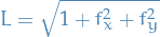
![\begin{equation*}
S[f] = \int_D \sqrt{1 + f_x^2 + f_y^2} \dd{x} \dd{y}
\end{equation*}](../../assets/latex/variational_calculus_134fc012886f41a9f8141e4647ed8e0b51ee8129.png)
If is an extremal of this function, we say that  is a minimal surface.
In this case the Lagrangian is
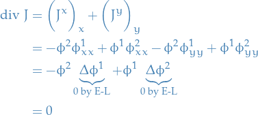
with the EL-equations
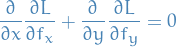
where
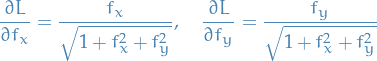
Therefore,
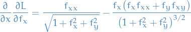
and similarily for . When combined, and multiplied by  since the combination equal zero anyways, we're left with

where we've used the fact that  .
.
This is then the equation which must be satisfied by a minimal surface.
 model
model
Noether's current for multidimensional Lagrangian
Classical Field Theory
Notation
 denotes a field written
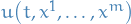

Concerned with action functionals of the form
![\begin{equation*}
S[u] = \int_{\Omega} \mathcal{L} \big( u, \nabla u, x \big) \dd[m + 1]{x}
\end{equation*}](../../assets/latex/variational_calculus_da40476f6f1a97534fc265ad98ebf491fd3b7a2e.png)
where
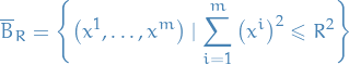
is called a Lagrangian density and ![$\Omega: [0, 1] \times \mathbb{R}^m$](../../assets/latex/variational_calculus_ebe396bb1a6f24062cd8e1e239e9cb7e712c1254.png) , i.e.
, i.e.
![\begin{equation*}
\Omega := \left\{ \big( x^0, x^1, \dots, x^m \big) \in \mathbb{R}^{m + 1} \mid x^0 \in [0, 1] \right\}
\end{equation*}](../../assets/latex/variational_calculus_af24f4e4fc73813190c1eee8f1833868f4265075.png)
 for
for  for some
  and
and

 denotes a "cylindrical" region
![\begin{equation*}
C_R = [a, b] \times \overline{B}_R \subset \Omega
\end{equation*}](../../assets/latex/variational_calculus_70a2fba565df2ebf857f830553012f410992e79f.png)
- is the outward normal to the boundary
Stuff
Lagrangian density is just used to refer to the fact that we are now looking at a variation of the form
![\begin{equation*}
S[x] = \int \mathcal{L} \dd[m + 1]{x} = \int \underbrace{\bigg( \int \mathcal{L} \dd[m]{x} \bigg)}_{= L} \dd{t}
\end{equation*}](../../assets/latex/variational_calculus_f55fbb2c6f8067422fe62347217042071ab23afe.png)
So it's like the ![$\int \mathcal{L} \dd[m]{x}$](../../assets/latex/variational_calculus_9af7de355d561c04b7e6b2f8769d8a5f4c7e8c51.png) is the Lagrangian now, and the "inner" functional is the a Lagrangian density.
is the Lagrangian now, and the "inner" functional is the a Lagrangian density.
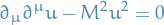
Klein-Gordon equation in  (i.e.
(i.e.  ) is given by
![\begin{equation*}
\pdv[2]{u}{\big( x^0 \big)} - \sum_{i=1}^{3} \pdv[2]{u}{\big( x^i \big)} + M^2 u = 0
\end{equation*}](../../assets/latex/variational_calculus_2f5d3eb6b5afbc6f845369f176edb20d8145bcc3.png)
where  is called the mass.
If  , then this is the wave equation, whence the Klein-Gordon equation is a sort of massive wave equation.
More succinctly, introducing the matrix
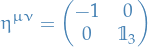
then the Klein-Gordon equation can be written
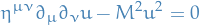
Note: you sometimes might see this written
where they use the notation  so we have sort of "summed out" the
  .
.
Calculus of variations with improper integrals
 is unbounded, and so we need to consider
![\begin{equation*}
S[u] = \lim_{R \to \infty} \int_{\Omega_R} \mathcal{L} \big( u, \nabla u, x \big) \dd[m + 1]{x}
\end{equation*}](../../assets/latex/variational_calculus_8c256b23450fd5b173d4eae555c80e97c2a46beb.png)
![$\Omega_R = [0, 1] \times \overline{B}_R$](../../assets/latex/variational_calculus_ac7351aed4fb8aaebe4e68c510d053d35a76f9b1.png) where
where
i.e. the closed ball of radius
Vary the action
![\begin{equation*}
\begin{split}
\dv{}{s} \bigg|_{s = 0} S[u + s \varepsilon] &= \lim_{R \to \infty} \int_{\Omega_R} \dv{}{s} \bigg|_{s = 0} \mathcal{L} \big( u + s \varepsilon, \nabla u + s \nabla e, x \big) \dd[m + 1]{x} \\
&= \lim_{R \to \infty} \int_{\Omega_R} \bigg( \pdv{\mathcal{L}}{u^i} \varepsilon^i + \pdv{\mathcal{L}}{u_{\mu}^i} \partial_{\mu} \varepsilon^i \bigg) \dd[m + 1]{x} \\
&= \lim_{R \to \infty} \int_{\Omega_R} \bigg( \pdv{\mathcal{L}}{u^i} - \partial_{\mu} \pdv{\mathcal{L}}{u_{\mu}^i} \bigg) \varepsilon^i \dd[m + 1]{x}
\end{split}
\end{equation*}](../../assets/latex/variational_calculus_ce0f891afbbcfd453e91c782b45000651226d1d8.png)
where we have omitted the boundary term
![\begin{equation*}
\lim_{R \to \infty} \int_{\Omega} \partial_{\mu} \pdv{\mathcal{L}}{u_{\mu}^i} \varepsilon^i \dd[m + 1]{x} = 0
\end{equation*}](../../assets/latex/variational_calculus_55dd13f05bb1fa38c861c015a66e165ee83f3688.png)
which is seen by applying the Divergence Theorem and using the BCs on the variation
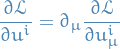
Using Fundamental Lemma of Calculus of Variations we obtain the E-L equations
Noether's Theorem for improper actions
- Consider action function for a classical field
 which is invariant under continuous one-parameter symmetry with Noether current
Integrate (zero) divergence of the current on a "cylindrical region"
![$C_R = [a, b] \times \overline{B}_R \subseteq \Omega$](../../assets/latex/variational_calculus_1a14f3420d2869c16ed86ed6343563dab4401e01.png) and apply the Divergence Theorem
and apply the Divergence Theorem
![\begin{equation*}
0 = \int_{C_R} \partial_{\mu} J^{\mu} \dd[m + 1]{x} = \int_{\partial C_R} N_{\mu} J^{\mu} \dd[m]{x}
\end{equation*}](../../assets/latex/variational_calculus_ec47df5d863e059661fe77b98ca453b9a5e868ec.png)
 consists of "sides"
 ![$[a, b] \times S_R^m$](../../assets/latex/variational_calculus_5da92e49234ca48729a2320a4fc162c4b53d1097.png) of the "cylinder", where
of the "cylinder", where
 is the m-sphere of radius
 - top cap

- bottom cap

Can rewrite the above as
![\begin{equation*}
\begin{split}
0 &= \int_{\overline{B}_R} J^0 \big( b, x^1, \dots, x^m \big) \dd[m]{x} - \int_{\overline{B}_R} J^0 \big( a, x^1, \dots, x^m \big) \dd[m]{x} \\
& \qquad + \underbrace{\int_{a}^{b} \int_{S_R^m} N^{\mu} J^{\mu} \big( x^0, x^1, \dots, x^m \big) \dd[m + 1]{x}}_{\to 0 \text{ as } R \to \infty}
\end{split}
\end{equation*}](../../assets/latex/variational_calculus_c63fcdfcbc9e109bea5e0beac2d261f7fb07aaca.png)
using the fact that
points outward at the bottom cap → negative  axis
axis
- Last term vanishes due to BCs on the field implies
 on as
on as 
- Last term vanishes due to BCs on the field implies
Since
 arbitrary, we have
![\begin{equation*}
Q = \lim_{R \to \infty} \int_{\overline{B}_R} J^0 \big( t, x^1, \dots, x^m \big) \dd[m]{x}
\end{equation*}](../../assets/latex/variational_calculus_04da75195107e8c19d1331ce1827a99c9a0367c3.png)
is conserved, i.e. we have a Noether's charge for the improper case!
Maxwell equations
Notation
 is the magnetic field
 is the electric field
 is the electric charge density
 is the electric current density
 is the magnetic potential
Let

Stuff
Maxwell's equations
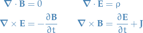
Observe that
 can be solved by writing
Does not determine
uniquely since

leaves
unchanged (since  ), and is called a gauge transformation
Substituting
 into Maxwell's equations:

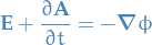
Thus there exists a function
 (again since ), called the electric potential, such that
Performing gauge transformation → changes
and unless also transform
In summary, two of Maxwell's equations can be solved by
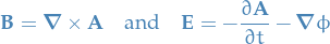
where
and are defined up to gauge transformations
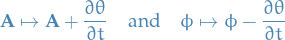
for some function

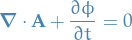
- We can fix the "gauge freedom" (i.e. limit the space of functions
 ) by imposing restrictions on , which often referred to as a choice of gauge, e.g. Lorenz gauge
- We can fix the "gauge freedom" (i.e. limit the space of functions
The ambiguity in the definition of and in the Maxwell's equations can be exploited to impose the Lorenz gauge condition:
In which case the remaining two Maxwell equations become wave equations with "sources":
![\begin{equation*}
\pdv[2]{\phi}{t} - \nabla^2 \phi = \rho \quad \text{and} \quad \pdv[2]{\mathbf{A}}{t} - \nabla^2 \mathbf{A} = \mathbf{J}
\end{equation*}](../../assets/latex/variational_calculus_3f9f9a3e10feb3277c5d61de8f3d7f546ca29fc3.png)
From these wave-equations we get electromagnetic waves!
Maxwell's equations are variational
- Let
 and
and  at first
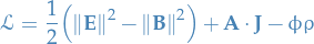
 Consider Lagrangian density
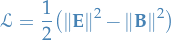
as functions of
and , i.e.
![\begin{equation*}
\mathcal{L} = \frac{1}{2} \bigg[ \big( \partial_i \phi \big)^2 + \big( \partial_t A_i \big)^2 + 2 \big( \partial_i \phi \big) \big( \partial_t A_i \big) \bigg] - \frac{1}{2} \bigg[ \big( \partial_i A_j \big)^2 - \big( \partial_i A_j \big)\big( \partial_j A_i \big) \bigg]
\end{equation*}](../../assets/latex/variational_calculus_6704ebb8469f931a7d4137df4a215df9025cdc53.png)
Observe that
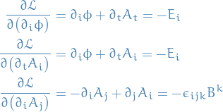
- does not depend explicitly on or , only on their derivatives, so E-L are
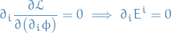
and
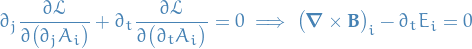
which are precisely the two remaining Maxwell equations when
and .
We can obtain the Maxwell equations with and nonzero by modifying :
We can rewrite by introducing the electromagnetic 4-potential
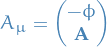
with  so that
  .
.
The electromagnetic 4-current is defined

so that  .
.
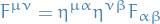
We define the fieldstrength

which obeys  .
.
We can think of  as entries of the
  antisymmetric matrix
![\begin{equation*}
\big[ F_{\mu \nu} \big] =
\begin{pmatrix}
0 & -E_1 & - E_2 & -E_3 \\
E_1 & 0 & B_3 & - B_2 \\
E_2 & - B_3 & 0 & B_1 \\
E_3 & B_2 & - B_1 & 0
\end{pmatrix}
\end{equation*}](../../assets/latex/variational_calculus_0d7dd977172ec6a04ecd02a0e831f93f9a8968a2.png)
where we have used that

In the terms of the fieldstrength we can write Maxwell's equations as
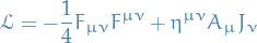
where we have used the "raised indices" of with  as follows:
The Euler-Lagrange equations of are given by

and the gauge transformations are

under which are invariant.
In the absence of sources, so when  , is gauge invariant.
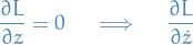
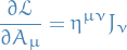
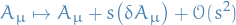
Let denote the action corresponding to , then
![\begin{equation*}
\dv{}{s}\bigg|_{s = 0} I \big[ A_{\mu} + s \varepsilon_{\mu} \big] = 0 \quad \iff \quad \pdv{\mathcal{L}}{A_{\mu}} = \pdv{}{x^{\nu}} \pdv{\mathcal{L}}{\big( \partial_{\nu} A_{\mu} \big)}
\end{equation*}](../../assets/latex/variational_calculus_05a895f0d4f852029d715641709f92b3a6369f9e.png)
where
and
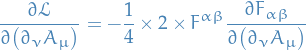
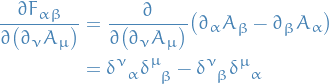
Therefore,
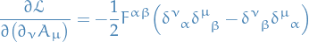
Substituing this into our E-L equations from above, we (apparently) get

In the absence of sources, so when , is gauge invariant. This is seen by only considering the second-order of the transformation
- First show that is invariant under the following
Consider
where

and

then

- Find the Nother currents
 and
and 
Examples
The Kepler Problem
- Illustrates Noether's Theorem and some techniques for the calculation of Poisson brackets
- Will set up problem both from a Lagrangian and a Hamiltonian point of view and show how to solve the system by exploiting conserved quantities
Notation
- Two particles of masses
 and
and  moving in
  , with
  and
and  denoting the corresponding positions
 - Assuming particles cannot occupy same position at same time, i.e.
 for all .
 We then have the total kinetic energy of the system given by
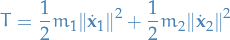
and potential energy
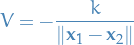
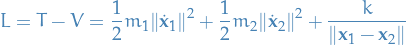
Lagrangian description
Lagrangian is, as usual given by
- is invariant under the diagonal action of the Euclidean group of on the configuration space, i.e. if
 is an orthonormal transformation and
  , then

leaves the Lagrangian invariant.