Differential Equations
Table of Contents
Stuff
Spectral method
A class of techniques to numerical solve certain differential equations. The idea is to write a solution of the differential equation as a sum of certain "basis functions" (e.g. Fourier Series which is a sum of sinouids) and then choose the coefficients in the sum in order to satisfy the differential equation as well as possible.
Series solutions
Definitions
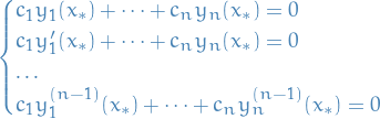
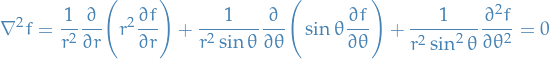
Suppose we have a second-order differential equation of the form

where  ,
,  and
and  are polynomials.
We then rewrite the equation as

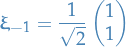
Then we say the point  is
is
- an ordinary point if the functions
 and
and  are analytic at
 - singular point if the functions aren't analytic
Convergence
Have a look at p. 248 in "Elementary Differential Equations and Boundary Problems". The two pages that follow summarizes a lot of different methods which can be used to determine convergence of a power series.
Systems of ODEs
Overview
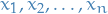
The main idea here is to transform some n-th order ODE into a system of  1st order ODEs, which we can the solve using "normal" linear algebra!
Procedure
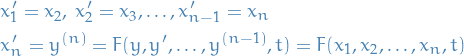
Consider an arbitrary n-th order ODE

- Change dependent variables to
 :
:

- Take derivatives of the new variables
Homogenous
Fundamental matrices
Suppose that 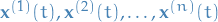 form a fundamental set of solutions for the equation

on some interval  . Then the matrix
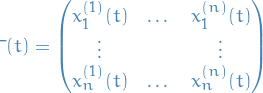
whose columns are the vectors , is said to be a fundamental matrix for the system.
Note that the fundamental matrix is nonsingular / invertible since the solutions are lin. indep.
We reserve the notation  for the fundament matrices of the form
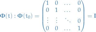
i.e. it's just a fundamental matrix parametrised in such a way that our initial conditions gives us the identity matrix.
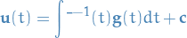
The solution of an IVP of the form:

can then be written

which can also be written
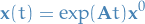
Finally, we note that

The exponential of a matrix is given by
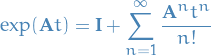
and we note that it satisfies differential equations of the form

since
![\begin{equation*}
\frac{d}{dt} [ \exp(\mathbf{A} t) ] = \sum_{n=1}^{\infty} \frac{\mathbf{A}^n t^{n-1}}{(n - 1)!} = \mathbf{A} \Bigg[ \mathbf{I} + \sum_{n=1}^{\infty} \frac{\mathbf{A}^n t^n}{n!} \Bigg] = \mathbf{A} \exp(\mathbf{A} t)
\end{equation*}](../../assets/latex/differential_equations_06d795474fca16fce328d45f50a633c5620b8197.png)
Hence, we can write the solution of the above differential equation as
Repeating eigenvalues
Suppose we have a repeating eigenvalue  (of algebraic multiplicity 2), with the found solution correspondig to
  is
is

where  satisfies

We then assume the other solution to be of the form

where  is determined by the equation

Multiplying both sides by  we get
since  by definition. Solving the above equation for and substituting that solution into the expression for
  we get the second solution corresponding to the repeated eigenvalue.
We call the vector the generalized eigenvector of  .
.
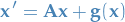
Non-homogenous
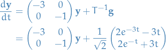
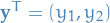
We want to solve the ODE systems of the form
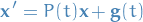
Which has a general solution of the form
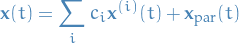
where 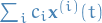 is the general solution to the corresponding homogenous ODE system.
We discuss the three methods of solving this:
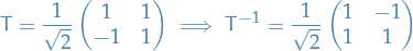
Diagonolisation
We assume the corresponding homogenous system is solved with the eigenvalues  and eigenvectors
  , and then introduce the change of variables
  :
:
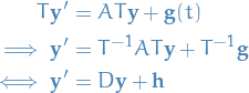
which gives us a system of decoupled systems:

and finally we transform back to the original variables:
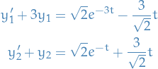
- Example
Consider
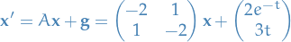
Since the system is linear and non-homogeneous, the general solution must be of the form
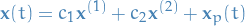
where
 denotes the particular solution.
The homogenous solution can be found as follows:
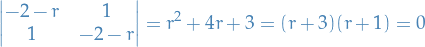
When
 : if
: if 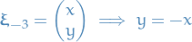 , hence we choose

When
 : if
: if 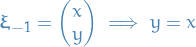 , hence we choose
Thus, the general homogenous solution is:

To find the particular solution, we make the change of variables
 :
:
With the new variables the ODE looks as follows:
Which in terms of
 is
is
Which, by the use of undetermined coefficients, we can solve as
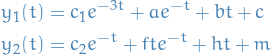
Doing "some" algebra, we eventually get
Then, finally, substituting back into the equation for
, and we would get the final result.
Undetermined coefficients
This method only works if the coefficient matrix  for some constant matrix , and the components of
  are polynomial, exponential, or sinusoidal functions, or sums or products of these.
Variation of parameters
This is the most general way of doing this.
Suppose we have the n-th order linear differential equation
![\begin{equation*}
L[y] = y^{(n)} + p_1(t) y^{(n - 1)} + \dots + p_{n - 1}(t) y' + p_n(t)y = g(t)
\end{equation*}](../../assets/latex/differential_equations_7b69465c5ec334852dc1292a5f0c7f52ff8f68ae.png)
Suppose we have found the solutions to the corresponding homogenous diff. eqn.

With the method of variation of parameters we seek a particular solution of the form

Since we have functions  to determine we have to specify conditions.
One of these conditions is cleary that we need to satisfy the non-homongenous diff. eqn. above. Then the  other conditions are chosen to make the computations as simple as possible.
Taking the first partial derivative wrt.  of
of  we get (using the product rule)

We can hardly expect it to be simpler to determine if we have to solve diff. eqns. of higher order than what we started out with; hence we try to surpress the terms that lead to higher derivatives of  by imposing the following condition
which we can do since we're just looking for some arbitrary functions  . The expression for
  then reduces to
Continuing this process for the derivatives  we obtain our condtions:

giving us the expression for the m-th derivative of to be

Finally, imposing that  has to satisfy the original non-homogenous diff. eqn. we take the derivative of
  and substitute back into the equation. Doing this, and grouping terms involving each of
  together with their derivatives, most of the terms drop out due to being a solution to the homogenous diff. eqn., yielding
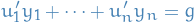
Together with the previous conditons we end up with a system of linear equations
(note the  at the end!).
The sufficient condition for the existence of a solution of the system of equations is that the determinant of coefficients is nonzero for each value of . However, this is guaranteed since  form a fundamental set of solutions for the homogenous eqn.
In fact, using Cramers rule we can write the solution of the system of equations in the form
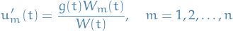
where  is the determinant of obtained from
  by replacing the m-th column by
  . This gives us the particular solution
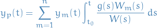
where  is arbitrary.
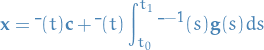
Assume that a fundamental matrix  for the corresponding homogenous system

has been found. We can then use the method of variation of parameters to construct a particular solution, and hence the general solution, of the non-homogenous system.
The general solution to the homogenous system is  , we seek a solution to the non-homogenous system by replacing the constant vector
  by a vector function
  . Thus we assume that

is a solution, where is a vector function to be found.
Upon differentiating  we get

Since is a fundamental matrix, 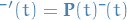 ; hence the above expression reduces to
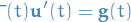
Since is nonsingular (i.e. invertible) on any interval where  is continuous. Hence
  exists, and therefore
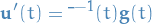
Thus for we can select any vector from the class of vectors which satisfy the previous equation. These vectors are determined only up to an arbitrary additive constant vector; therefore, we denote by
where the constant vector is arbitrary.
Finally, this gives us the general solution for a non-homogenous system
Dynamical systems
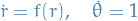
In  , an arbitrary autonomous dynamical system can be written as

for some smooth  , for a the 2D case:
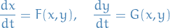
which in matrix notation we write
Notation
 denotes a critical point
 denotes the RHS of the autonomous system
 denotes a specific solution
Theorems
The critical point  of the linear system
where we suppose has eigenvalues  , is:
, is:
- asymptotically stable if are real and negative
- stable if are pure imaginary
- unstable if are real and either positive, or have positive real part
Stability
The points  are called critical points of the autonomous system

Let be a critical point of the system.
- is said to be stable if for any
 ,
,

for all
 .
I.e. for some solution
.
I.e. for some solution  we parametrize it such that
  for some
  such that we stay close to for all , then we say it's stable.
- is said to be asymptotically stable if it's stable and there exists a
 s.t. that if a solution satisfies
then
i.e. if we start near
, the limiting behaviour converges to . Note that this is stronger than just being stable.
- which is NOT stable, is of course unstable.
Intuitively what we're saying here is that:
- for any we can find a trajectory (i.e. solution with a specific initial condition, thus we can find some initial condition ) such that the entire trajectory stays within of the critical points for all
 .
.
When we say a critical point is isolated, we mean that there are no other critical points "nearby".
In the case of a system
By solving the equation

if the solution is a single vector, rather than a line or plane, the critical point is not isolated.
Suppose that we have the system
and that is a isolated critical point of the system. We also assume that  so that is also a isolated critical point of the linear system
  . If
. If
that is,  is small in comparison to
  near the critical point , we say the system is a locally linear system in the neighborhood of the critical point .
Linearized system
In the case where we have a locally linear system, we can approximate the system near isolated critical points by instead considering the Jacobian of the system. That is, if we have the dynamical system
with a critical point at  , we can use the linear approximation of
  near :

where  denotes the Jacobian of , which is
Substituting back into the ODE

Letting  , we can rewrite this as

which, since  is constant given , gives us a linear ODE wrt
  , hence the name linearization of the dynamical system.
Hopefully  is a simpler expression than what we started out with.
General procedure
- Obtain critical points, i.e.

- If non-linear and locally linear, compute the Jacobian and use this is an linear approximation to the non-linear system, otherwise: do nothing.
- Inspect the following to determine the behavior of the system:
 and
and 
- Compute eigenvalues and eigenvectors to obtain solution of the (locally) linear system
- Consider asymptotic behavior of the different terms in the general solution, i.e.

 which provides insight into the phase diagram / surface. If non-linear, first do for linear approx., then for non-linear system
Points of interest
The following section is a very short summary of Ch. 9.1 [Boyce, 2013]. Look here for a deeper look into what's going on, AND some nice pictures!
Here we consider 2D systems of 1st order linear homogenous equations with constant coefficients:

where  and
and  . Suppose are the eigenvalues for the matrix , and thus gives us the expontentials for the solution
  .
.
We have multiple different cases which we can analyse:
 :
:
- Exponential decay: node or nodal sink
- Exponential growth. node or nodal source
 : saddle point
 :
:
- two independent eigenvectors: proper node (sometimes a star point )
- one independent eigenvector: improper or degenerate node
 : spiral point
- spiral sink refers to decaying spiral point
- spiral source refers to growing spiral point
 : center
Basin of attraction
This denotes the set of all points in the xy-plane s.t. the trajectory passing through approaches the critical point as  .
.
A trajectory that bounds the basin of attraction is called a separatix.
Limit cycle
Limit cycles are periodic solutions such that at least one other non-closed trajectory asymptotes to them as and / or  .
.
Let  and
and  have continuous first partial derivatives in a simply connected domain
  .
.
If  has the same sign in the entire , then there are no closed trajectories in .
Consider the system

Let and have continious first partial derivatives in a domain .
Let  be a bounded subdomain of and let
  .
Suppose contains no critical points.
.
Suppose contains no critical points.
If

then
- solution is periodic (closed trajectory)
- OR it spirals towards a closed trajectory
Hence, there exists a closed trajectory.
Where
- denotes a particular trajectory
 denotes the boundary of
Useful stuff
- Example
Say we have the following system:
where
 , has periodic solutions corresponding to the zeroes of
  .
What is the direction of the motion on the closed trajectories in the phase plane?
.
What is the direction of the motion on the closed trajectories in the phase plane?
Using the identities above, we can rewrite the system as
Which tells us that the trajectories are moving in counter-clockwise direction.
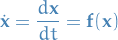
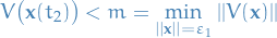
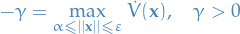
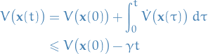
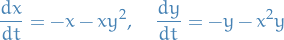
Lyapunov's Second Method
Goal is to obtain information about the stability or instability of the system without explicitly obtaining the solutions of the system. This method allows us to do exactly that through the construction of a suitable auxillary function, called the Lyapunov function.
For the 2D-case, we consider such a function of the following form:

where and are as given in the autonomous system definition.
We choose the notation above because  can be identified as the rate of change of
  along the trajectory of the system that passes through the point
  . That is, if
 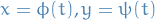 is a solution of the system, then
![\begin{equation*}
\begin{split}
\frac{d V[\phi(t), \psi(t)]}{d t} &= V_x [\phi(t), \psi(t)] \frac{d \phi(t)}{dt} + V_y [\phi(t), \psi(t)] \frac{d \psi(t)}{dt} \\
&= V_x(x, y) F(x, y) + V_y(x, y) G(x, y) \\
&= \dot{V}(x, y)
\end{split}
\end{equation*}](../../assets/latex/differential_equations_eb6d5d1753dd4ece351488567e383c226b6440d5.png)
Suppose that the autonomous system has an isolated critical point at the origin.
If there exists a continuous and positive definite function which also has continuous first partial derivatives :
- if
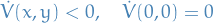 ( negative definite ) on some domain , then the origin is an asymptotically stable critical point
 - if
 ( negative semidefinite ) then the origin is a stable point
Suppose that the autonomous system has an isolated critical point at the origin.
Let be a function that is continuous and has continuous first partial derivatives.
Suppose that  and that in every neighborhood of the origin there is a least one point at which is positive (negative). If there exists a domain containing the origin such that the function is positive definite ( negative definite ) on , then the origin is an unstable point.
Let the origin be an isolated critical point of the autonomous system. Let the function be continous and have continuous first partial derivatives. If there is a bounded domain  containing the origin where
  for some positive
  , is positive definite and is negative definite , and then every solution of the system that starts at a point in approaches the origin as .
We're not told how to construct such a function. In the case of a physical system, the actual energy function would work, but in general it's more trial-and-error.
Lyapunov function
Lyapunov functions are scalar functions which can be used to prove stability of an equilibrium of an ODE.
Lyapunov's Second Method (alternative)
Notation
Definitions
Let  be a continuous scalar function.
is a Lyapunov-candidate-function if it's /locally positive-definite function, i.e.

with  bein a neighborhood region around
  .
.
Further, let  be a critical or equilibrium point of the autonomous system
And let

Then, we say that the Lyapunov-candidate-function  is a Lyapunov function of the system if and only if
where denotes a specific trajectory of the system.
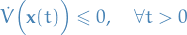
For a given autonomous system, if there exists a Lyapunov function in some neigborhood of some critical / equilibrium point , then the system is stable (in a Lyapunov sense).
Further, if is negative-definite, i.e. we have a strict inequality
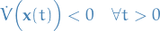
then the system is asymptotically stable about the critical / equilibrium point .
When talking about critical / equilibrium point , when considering a Lyapunov function, we have to make sure that the critical point corresponds to . This can easily be achieved by "centering" the system about the point original critical point , i.e. creating some new system with  , which will then have the corresponding critical point at
  .
.
Observe that this in no way affects the qualitative analysis of the critical point.
Let be a continuous scalar function.
is a Lyapunov-candidate-function if it's a locally postitive-definite function, i.e.

with being a neighborhood region around .
Let be a critical / equilibrium point of the autonomous system
And let

be the time-derivative of the Lyapunov-candidate-function .
Let be a locally positive definite function (a candidate Lyapunov function) and let be its derivative wrt. time along the trajectories of the system.
If is locally negative semi-definite, then is called a Lyapunov function of the system.
If there exists a Lyapunov function  of a system, then
  is a stable equilibrium point in the sense of Lyapunov.
If in addition  and
and  for some
  , i.e. is locally negative definite , then is asymptotically stable.
Remember, we can always re-parametrize a system to be centered around a critical point, and come to an equivalent analysis of the system about the critical point, since we're simply "adding" a constant.
Proof
First we want to prove that if is a Lyapunov function then is a stable critical point.
Suppose is given. We need to find such that for all  , it follows that
  .
.
Then let  , where
  is the radius of a ball describing the "neighborhood" were we know that is a Lyapunov candidate function, and define
Since is continuous, the above  is well-defined and positive.
Choose  satisfying
  such that for all
  . Such a choise is always possible, again because of the continuity of .
Now, consider any  such that
  and thus
  and let be the resulting trajectory. Observe that
  is non-increasing, that is

which results in  .
.
We will now show that this implies that  , for a trajectory defined such that and thus
  as described above.
Suppose there exists  such that
  , then since we're assuming is such that

as described above, then clearly we also have

Further, by continuity (more specifically, the IVT) we must have that at an earlier time  we had

But since  , we clearly have
due to  . But the above implies that
Which is a contradiction, since  implying that
 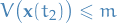 .
.
Now we prove the theorem for asymptotically stable solutions! As stated in the theorem, we're now assuming to be locall negative-definite, that is,

We then need to show that

which by continuity of , implies that  .
.
Since is strictly decreasing and  we know that

And we then want to show that  . We do this by /contradiction.
Suppose that  . Let the set
  be defined as

and let  be a ball inside of radius
  , that is,

Suppose is a trajectory of the system that starts at .
We know that is decreasing monotonically to  and
and  for all . Therefore,
  , since
  which is defined as all elements for which
  (and to drive the point home, we just established that the ).
In the first part of the proof, we established that

We can define the largest derivative of as
Clearly,  since
since  is locally negative-definite. Observe that,
which implies that  , resulting in a contradiction established by the , hence .
Remember that in the last step where say suppose "there exists such that  " we've already assumed that the initial point of our trajectory, i.e. for , was within a distance
  from the critical point ! Thus we would have to cross the "boundary" defined by from .
Therefore, intuitively, we can think of the Lyapunov function providing a "boundary" which the solution will not cross given it starts with this "boundary"!
Side-notes
- When reading about this subject, often people will refer to Lyapunov stable or Lyapunov asymptotically stable , which is exactly the same as we define to be stable solutions.
Examples of finding Lyapunov functions
- Quadratic
The function

is positive definite if and only if

and is negative definite if and only if

- Example problem
Show that the critical point
 of the autonomous system
is asymptotically stable.
We try to construct a Liapunov function of the form
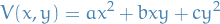
then

thus,
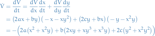
We observe that if we choose
 , and
, and  and to be positive numbers, then is negative-definite and is positive-definite. Hence, the critical point is asymptotically stable.
- Example problem
Partial Differential Equations
Consider the differential equation

with the boundary conditions
We call this a two-point boundary value problem.
This is in contrast to what we're used to, which is initial value problems, i.e. where the restrictions are on the initial value of the differential equation, rather than the boundaries of the differential equations.
Eigenvalues and eigenfunctions
Consider the problem consisting of the differential equation
together with the boundary conditions
By extension of terminology from linear algebra, we call each nontrivial (non-zero) constant  an eigenvalue and the corresponding nontrivial (not everywhere zero) solution
  an eigenfunction.
Specific functions
Heat equation
Models heat distribution in a row of length  .
.

with boundary conditions:

and initial conditions:

Wave equation
Models vertical displacement  wrt. horizontal position
  and time .
where  ,
,  being the tension in the string, and being the mass per unit length of the string material.
Reasonable to have the boundary conditions:

i.e. the ends of the string are fixed.
And the initial conditions:

i.e. we have some initial displacement  and initial (vertical) velocity
  . To keep our boundary condtions wrt. specified above consistent:

Laplace equation
or
Since we're dealing with multi-dimensional space, we have a couple of different ways to specify the boundary conditions:
- Dirichlet problem : the boundary of the surface takes on specific values, i.e. we have a function
 which specifies the values on the "edges" of the surface
 - Neumann problem : the values of the normal derivative are prescribed on the boundary
We don't have any initial conditions in this case, as there's no time-dependence.
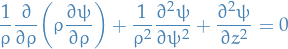
- Laplace's equation in cylindrical coordinates
Let

Laplace's equation becomes:
Consider BCs:

Using separation of variables:

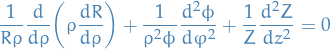
we can rewrite as:
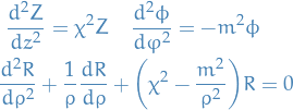
Using
 ,
,  , hence
Thus, if
 , solutions are periodic.
The radial equation can be written in the SL-form
Thus,
 : vanish at the origin
 : unbounded as
Finally, making the change of variables
 amd write
  , we have
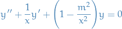
Which is the Bessel equation, and we have the general solution:

Imposing the boundary conditions:

 as needs to be bounded
 and
and  for
for 
 as (due to log)
Hence, we require

Plotting these Bessel functions, we conclude there exists a countable infinite number of eigenvalues.
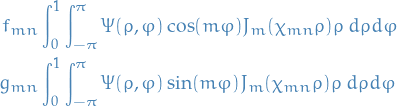
We now superpose the solutions:

to write the general solution as

The constants
 and
and  are found from the remaining BC,
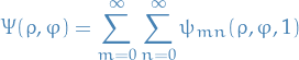
by projection on
 and
and  .
.
Orthogonality: the Besseul functions
 satisfy
![\begin{equation*}
L[R_{mn}] = - \big( \rho R_{mn}' \big)' + \frac{m^2}{\rho} R_{mn} = \rho \xi^2 R_{mn}
\end{equation*}](../../assets/latex/differential_equations_8f950103cc7e7560fe1814d4743ed339f931637a.png)
Which has the Sturm-Liouville form, with
![\begin{equation*}
\langle L[u], v \rangle = \langle u, L[v] \rangle
\end{equation*}](../../assets/latex/differential_equations_448eef7bf1a72722a6b39f061eea76d62cd8cc89.png)
provided that
![\begin{equation*}
0 = p(x) [u'v - u v']_0^1
\end{equation*}](../../assets/latex/differential_equations_6aca78d825f931fadae55549e4945366d173260a.png)
The functions
 satisfy the above at
  , where the contribution at vanishes,
and at we have
, where the contribution at vanishes,
and at we have
![\begin{equation*}
\lim_{\varepsilon \to 0} p(\varepsilon) [u'(\varepsilon)v(\varepsilon) - u(\varepsilon)v'(\varepsilon)] = 0
\end{equation*}](../../assets/latex/differential_equations_603421dd8547e6df0eaf5410be172964312ab140.png)
since
 and
and  and
and  are bounded.
We conclude
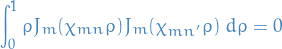
for
 . We can therefore identify the constants and by projection:
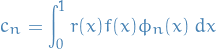
Boundary Value Problems and Sturm-Liouville Theory
Notation
![$L[y] = - [p(x) y']' + q(x) y$](../../assets/latex/differential_equations_ffa3173a593a95d2d82ccb2156f377dee8b5f737.png)
 are the ordered eigenvalues
 are the corresponding normalized eigenfunctions
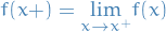 and equivalent for
Sturm-Liouville BVP
Equation of the form:
![\begin{equation*}
[p(x) y']' - q(x) y + \lambda r(x) y = 0
\end{equation*}](../../assets/latex/differential_equations_98a26130aba7476ead15479889726738075ec5c1.png)
OR equivalently
![\begin{equation*}
L[y] = \lambda r(x) y
\end{equation*}](../../assets/latex/differential_equations_03fa7e9cf8a0b1ef8849178876934fbcd61eb076.png)
with boundary conditions:

where we the boundary value problem to be regular, i.e.:
 and are continuous on the interval
 ![$[0, 1]$](../../assets/latex/differential_equations_68c8fa38d960e53d4308cbf1e65d04c66a554817.png)
 and
and  for all
 ![$x \in [0, 1]$](../../assets/latex/differential_equations_1abcf6a6ba0996351c652ec55b2a137f25774cfc.png)
and the boundary conditions to be separated, i.e.:
- each involves only on the of the boundary points
- these are the most general boundary conditions you can have for a 2nd order differential equation
Lagrange's Identity
Let  and
and  be functions having continous second derivatives on the interval , then
![\begin{equation*}
\int_0^1 L[u] \ v \ dx = \int_0^1 [- (pu')' v + quv ] \ dx
\end{equation*}](../../assets/latex/differential_equations_ff6cee08b44f949777f46fcd7f3ea126a06db06d.png)
where ![$L[y]$](../../assets/latex/differential_equations_649363683ef118ca5d298ad11b129363dc829bbd.png) is given by
is given by
![\begin{equation*}
L[y] = - [p(x) y']' + q(x) y
\end{equation*}](../../assets/latex/differential_equations_922b2cd49b7c861e86e8af3a1142195d7571cc2d.png)
In the case of a Sturm-Liouville problem we have observe that the Lagrange's identity gives us
![\begin{equation*}
\int_0^1 L[u] v - u L[v] \ dx = - p(x) [u'(x) v(x) - u(x) v'(x)] \Big|_0^1
\end{equation*}](../../assets/latex/differential_equations_adfd03b9802dce88d6cba9cf6ef1aba2fd9c93ac.png)
Which we can expand to
![\begin{equation*}
- p(x) [u'(x) v(x) - u(x) v'(x)] \Big|_0^1 = - p(1) [u'(1) v(1) - u(1) v'(1)] + p(0) [u'(0)v(0) - u(0)v'(0)]
\end{equation*}](../../assets/latex/differential_equations_28af542a94ae9b9e1aecb8a68273b43bc95e65ae.png)
Now, using the boundary conditions from the Sturm-Liouville problem, and assuming that  and
and  , we get
![\begin{equation*}
\begin{split}
- p(x) [u'(x) v(x) - u(x) v'(x)] \Big|_0^1 &= - p(1) \Bigg[\frac{\beta_1}{\beta_2} u(1) v(1) - u(1) \frac{\beta_1}{\beta_2} v(1) \Bigg] + \Bigg[\frac{\alpha_1}{\alpha_2} u(1) v(1) - u(1) \frac{\alpha_1}{\alpha_2} v(1) \Bigg] \\
&= 0
\end{split}
\end{equation*}](../../assets/latex/differential_equations_0afd70dadfa639f4cd067c4fcb65ddad21f905a9.png)
And if either  or
or  are zero,
  or
or  and the statement still holds.
I.e. the Lagrange's identity under the Sturm-Liouville boundary conditions equals zero.
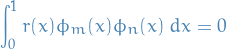
If  are solutions to a boundary value problem of the form def:sturm-lioville-problem, then
![\begin{equation*}
\int_0^1 L[u] v - u L[v] \ dx = 0
\end{equation*}](../../assets/latex/differential_equations_95d49fde485f96fd9ac6dca7cb0938401949cd8e.png)
or in the form of an inner product
![\begin{equation*}
\langle L[u], v \rangle - \langle u, L[v] \rangle = 0
\end{equation*}](../../assets/latex/differential_equations_a7ee36585ff183bc1e5808e827977a90823d5dd2.png)
If a singular boundary value problem of the form def:sturm-lioville-problem satisfies thm:lagranges-identity-sturm-liouville-boundary-conditions then we say the problem is self-adjoint. More specifically,
for an n-th order operator
![\begin{equation*}
L[y] = p_n(x) \frac{d^n y}{dx^n} + \dots + p_1(x) \frac{dy}{dx} + p_0(x) y
\end{equation*}](../../assets/latex/differential_equations_64da7f6d6ce823557626d751453160e7c57a606b.png)
subject to linear homogenous boundary conditions at the endpoints is self-adjoint provided that
![\begin{equation*}
\langle L[u], v \rangle - \langle u, L[v] \rangle = 0
\end{equation*}](../../assets/latex/differential_equations_e95393597b3a6d1e6cdd3eca6017fd8a1da7ec29.png)
E.g. for 4th order we can have
![\begin{equation*}
L[y] = \big[ p(x) y'' \big]'' - [q(x) y']' + s(x) y
\end{equation*}](../../assets/latex/differential_equations_a8874d9e50da5a385bfabaee7d02f39dcbe9bb2a.png)
plus suitable BCs.
Most results from the 2nd order problems extends to the n-th order problems.
Some theorems
All the eigenvalues of the Sturm-Liouville problem are real.
If  and
and  are two eigenfunctions of the Sturm-Lioville problem corresponding to the eigevalues
  and
and  , respectively, and if
  , then
That is, the eigenfunctions  are *orthogonal to each other wrt. the weight function
  .
.
We note that and , with , satisfy the differential equations
![\begin{equation*}
L[\phi_m] = \lambda_m r \phi_m
\end{equation*}](../../assets/latex/differential_equations_19e61c777151bfafd1abfc18e7d8e634e2a563cc.png)
and
![\begin{equation*}
L[\phi_n] = \lambda_n r \phi_n
\end{equation*}](../../assets/latex/differential_equations_2606a4e130d128c7e11e6419d49b17a749c6f95d.png)
respectively. If we let  and
and  , and substitute
 ![$L[u]$](../../assets/latex/differential_equations_0355559536e6c9a484e534051de4eef9e1a80d9b.png) and
and ![$L[v]$](../../assets/latex/differential_equations_7ba08366b1b41b349e411a74c92e6007514287a0.png) into Lagrange's Identity with Sturm-Liouville boundary conditions, we get
into Lagrange's Identity with Sturm-Liouville boundary conditions, we get

which implies that  where
where  represents the inner-product wrt. .
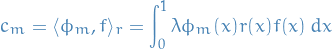
The above theorem has further consequences that, if some function  satisfies is continuous on , then we can expand as a linear combination of the eigenfunctions of the Sturm-Liouville equation!
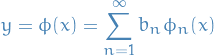
Let be the normalized eigenfunctions of the Sturm-Liouville problem.
Let and  be piecewise continuous on . Then the series
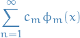
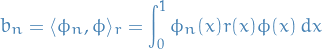
whose coefficients  are given by
converges to ![$[f(x+) + f(x-)] / 2$](../../assets/latex/differential_equations_18cdf0058c30358feb7f6fad00bc6685449b41a5.png) at each point in the open interval
at each point in the open interval  .
.
The eigenvalues of the Sturm-Liouville problem are all simple; that is, to each eigenvalue there corresponds only one linearly independent eigenfunction.
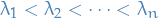
Further, the eigenvalues form an infinite sequence and can be ordered according to increasing magnitude so that
Moreover,  as
as  .
.
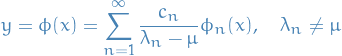
Non-homogenous Sturm-Liouville BVP
"Derivation"
Consider the BVP consisting of the nonhomogenous differential equation
![\begin{equation*}
L[y] = - [p(x) y']' + q(x) y = \mu r(x) y + f(x)
\end{equation*}](../../assets/latex/differential_equations_526d93dc3cd435b16042eb7835d6e609c75cb7c7.png)
where  is a given constant and is a given function on , and the boundary conditions are as in homogeonous Sturm-Lioville.
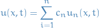
To find a solution to this non-homogenous case we're going to start by obtaining the solution for the corresponding homogenous system, i.e.
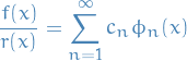
where we let be the eigenvalues and be the eigenfunctions of this differential equation. Suppose
i.e. we write the solution as a linear combination of the eigenfunctions.
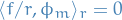
In the homogenous case we would now obtain the coefficients  by
by
which we're allowed to do as a result of the orthogonality of the eigenfunctions wrt. .
The problem here is that we actually don't know the eigenfunctions yet, hence we need a different approach.
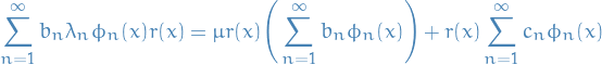
We now notice that  always satisfies the boundary conditions of the problem, since each does! Therefore we only need to deduce such that the differential equation is also satisifed. We start by substituing our expansion of into the LHS of the differential equation
![\begin{equation*}
L[\phi] = L \Bigg[ \sum_{n=1}^{\infty} b_n \phi_n(x) \Bigg] = \sum_{n=1}^{\infty} b_n L[\phi_n] = \sum_{n=1}^{\infty} b_n \lambda_n \phi_n(x) r(x)
\end{equation*}](../../assets/latex/differential_equations_7d3888e0c84011eb4fb78454bbdd334036437032.png)
since ![$L[\phi_n] = \lambda_n r \phi_n$](../../assets/latex/differential_equations_62cf2485194ec4c03febb3dc3a917bd243ef701c.png) from the homogenous SL-problem, where we have assumed that we interchange the operations of summations and differentiation.
from the homogenous SL-problem, where we have assumed that we interchange the operations of summations and differentiation.
Observing that the weight function occurs in all terms except  . We therefore decide to rewrite the nonhomogenous term as
 ![$r(x) [f(x) / r(x)]$](../../assets/latex/differential_equations_e2d7a786f857163fdcaee6f8d27084af0bd84863.png) , i.e.
, i.e.
![\begin{equation*}
L[\phi] = r(x) \phi(x) + r(x) \frac{f(x)}{r(x)}
\end{equation*}](../../assets/latex/differential_equations_44cf510d5218d0e52d6fba1f3f77d50436c31974.png)
If the function  satisfies the conditions in thm:boyce-11.2.4, we can expand it in the eigenfunctions:
where

Now, substituting this back into our differential equation we get
Dividing by , we get
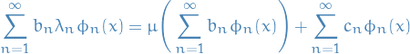
Collecting terms of the same we get
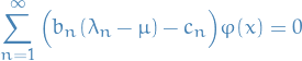
Now, for this to be true for all , we need each of the terms to equal zero. To make our life super-simple, we assume  for all , then
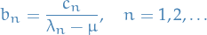
and thus,
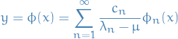
And remember, we already have an expression for  and know from the corresponding homogeonous problem.
If  for some then we have two possible cases:
 and thus there exists no solution of the form we just described
 in which case
 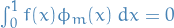 , thus we can only solve the problem if is orthogonal to ; in this case we have an infinite number of solutions since the m-th coefficient can be arbitrary.
Summary
![\begin{equation*}
L[y] = \mu \ r(x) y + f(x)
\end{equation*}](../../assets/latex/differential_equations_dd86144bf506d0aed4ef4c9504782b44ff7cf2eb.png)
with boundary conditions:

Expanding 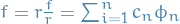 , which means that we can rewrite the diff. eqn. as
![\begin{equation*}
\begin{split}
L[\phi] &= \mu r \phi + \sum_{i=1}^{n} c_n \phi_n r \Big( \frac{f}{r} \Big) \\
L \Big[ \sum_{i=1}^{n} b_n \phi_n \Big] &=
\end{split}
\end{equation*}](../../assets/latex/differential_equations_2fa395dfa57dbc9dbfca4eb615f1b08e2518ce53.png)
We have the solution
where and  are the eigenvalues and eigenfunctions of the corresponding homogenous problem, and

If for some we have:
- in which case there exist no solution of the form described above
- i which case
 ; in this case we have an infinite number of solutions since the m-th coefficient can be arbitrary
Where we have made the following assumptions:
- Can rewrite the nonhomogenous part as
![$f(x) = r(x) \ [ f(x) / r(x) ]$](../../assets/latex/differential_equations_64231872871ce79f27540405ec60e365398313d1.png)
- Can expand
 using the eigenfunctions wrt. , which requires and to be continuous on the domain
Inhomogenous BCs Sturm-Liouville BVP
Derivation (sort-of-ish)
Consider we have at our hands a Sturm-Liouville problem of the sort:
![\begin{equation*}
\partial_{xx}^2 u - \beta^2 u = \partial_{tt}^2 u, \qquad x \in [0, a], \quad t > 0
\end{equation*}](../../assets/latex/differential_equations_6ff7fc38c4a41d467d2166bbf63581c438fee0d6.png)
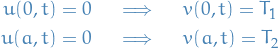
for any  , satisfying the boundary conditions
![\begin{equation*}
\begin{split}
u(0, t) = 0 &\quad u(a, t) = 0, \quad t > 0 \\
u(x, 0) = f(x), &\quad \partial_t u(x, 0) = 0, \quad \forall x \in [0, a]
\end{split}
\end{equation*}](../../assets/latex/differential_equations_3981b2b2cefa3fc6dd9c44466f3ea3944124cc52.png)
This is just a specific Sturm-Liouville problem we will use to motivate how to handle these inhomogenous boundary-conditions.
Suppose we've already obtained the solutions for the above SL-problem using separation of variables, and ended up with:

as the eigenfunctions, with the general solution:
where 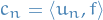 such that we satisfy the
  BC given above.
Then, suddenly, the examinator desires you to solve the system for a slightly different set of BCs:

What an arse, right?! Nonetheless, motivated by the potential of showing that you are not fooled by such simple trickeries, you assume a solution of the form:

where is just as you found previously for the homogenous BCs.
Eigenfunctions (i.e. (countable) infinite number of orthogonal solutions)) arise only in the case of homogenous BCs, as we then still have the Lagrange's identity being satisifed. For inhomogenous BCs, it's not satisfied, and we're not anymore working with a Sturm-Liouville problem.
Nonetheless, we're still solving differential equations, and so we still have the principle of superposition available to work with.
Why would you do that? Well, setting up the new BCs:
![\begin{equation*}
\begin{split}
w(0, t) = u(0, t) + v(0, t) = T_1 &\quad w(a, t) = u(a, t) + v(a, t) = T_2, \quad t > 0 \\
w(x, 0) = u(x, 0) + v(x, 0) = f(x), &\quad \partial_t w(x, 0) = \partial_t u(x, 0) + \partial_t v(x, 0) = 0, \quad \forall x \in [0, a]
\end{split}
\end{equation*}](../../assets/latex/differential_equations_aea4ac39c8606d562523ded42d12744faffb3935.png)
Now, we can then quickly observe that we have some quite major simplifications:
If we then go on to use separation of variables for  too, we have
Substituting into the simplified BCs we just obtained:

Here it becomes quite apparent that this can only work if  , and if we simply include this constant factor into our
  , we're left with the satisfactory simple expressions:

This is neat and all, but we're not quuite ready to throw gang-signs in front of the examinator in celebration quite yet. Our expression for the additional has now been reduced to
Substituting this into the differential equation (as we still of course have to satisfy this), we get
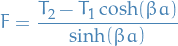
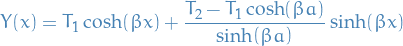
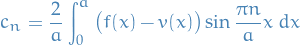
where the t-dependent factor has vanished due to our previous reasoning (magic!). Recalling that  , the general solution is simply

Substituting into the BCs from before:

where the last BC  gives us
thus,
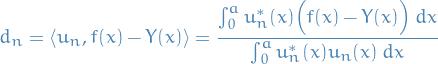
Great! We still have to satisfy the initial-values, i.e. the BCs for  . We observe that they have now become:

where the last t-dependent BC stays the same due to  being independent of . For the first BC, the implication arises from the fact that we cannot alter any further to accomodate the change to the complete solution, hence we alter . With this alteration, we end up with the complete and final solution to the inhomogenous boundary-condition problem
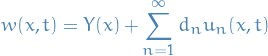
where
At this point it's fine to throw gang-signs and walk out.
Observe that is kept outside of the sum. It's a tiny tid-bit that might be forgotten in all of this mess: we're adding a function to the general solution to the "complete" PDE, that is

NOT something like this  .
.
I sort of did that right away.. But quickly realized I was being, uhmm, not-so-clever. Though I guess we could actually do it if we knew to be square-integrable! Buuut..yeah, I was still being not-so-clever.
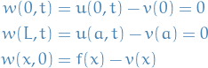
Example
Suppose we we're presented with a modified wave equation of the following form:
for any , satisfying the boundary conditions
and we found the general solution to be
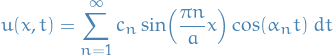
where is as given above.
Now, one might wanted, what would the solution be if we suddenly decided on a set of non-homogenous boundary conditions :

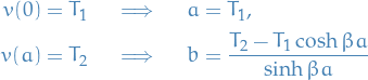
To deal with non-homogenous boundary conditions, we look for a time independent solution  solving the boundary problem

Once is known, we determine the solution to the modified wave equation using

where  satisfies the same modified equation with different initial conditions, but homogenous boundary conditions. Indeed,
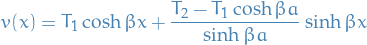
To determine , we solve the second order ODE with constant coefficients. Since , its general solution is given by

We fix the arbitrary constants using the given boundary conditions
Thus, the general solution is given by
By construction, the remaining is as in the previous section, but with the coefficients  satisfying
Thus, the very final solution is given by
with as given above.
Singular Sturm-Liouville Boundary Value Problems
We use the term singluar Sturm-Liouville problem to refer to a certain class of boundary value problems for the differential equation
![\begin{equation*}
L[y] = \lambda r(x) y, \quad 0 < x < 1
\end{equation*}](../../assets/latex/differential_equations_afbe22fc9b3fbdf5025b48bb9d3a6e97f31d1933.png)
in which the functions  and satisfy the conditions (same as in the "regular" Sturm-Liouville problem) on the open interval
  , but at least one of the functions fails to satisfy them at one or both of the boundary points.
Discussion
Here we're curious about the following questions:
- What type of boundary conditions can be allowed in a singular Sturm-Liouville problem?
- What's the same as in the regular Sturm-Liouville problem?
- Are the eigenvalues real?
- Are the eigenfunctions orthogonal?
- Can a given function be expanded as a series of eigenfunctions?
These questions are answered by studying Lagrange's identity again.
To be concrete we assume  is a singular point while
  is not.
Since the boundary value problem is singular at we choose and consider the improper integral
![\begin{equation*}
\int_{\varepsilon}^1 \{ L[u] v - u L[v] \} \ dx = - p(x) [ u'(x) v(x) - u(x) v'(x) ] \Big|_{\varepsilon}^{1}
\end{equation*}](../../assets/latex/differential_equations_2614cb9257962279df8f34af986adfd72ae137dd.png)
If we assume the boundary conditions at are still satisfied, then we end up with
![\begin{equation*}
\int_{\varepsilon}^1 \{ L[u] v - u L[v] \} \ dx = p(\varepsilon) [ u'(\varepsilon) v(\varepsilon) - u(\varepsilon) v'(\varepsilon)]
\end{equation*}](../../assets/latex/differential_equations_81ea7aa8c40b8b4e7f135eaff1f2890004396608.png)
Taking the limit as  :
:
![\begin{equation*}
\int_0^1 \{ L[u] v - u L[v] \} \ dx = \underset{\varepsilon \to 0}{\lim} \ p(\varepsilon) [ u'(\varepsilon) v(\varepsilon) - u(\varepsilon) v'(\varepsilon)]
\end{equation*}](../../assets/latex/differential_equations_7aaae5dacb800f4ba4207ef4be127ed82fc5cf56.png)
Therefore, if we have
![\begin{equation*}
\underset{\varepsilon \to 0}{\lim} \ p(\varepsilon) [ u'(\varepsilon) v(\varepsilon) - u(\varepsilon) v'(\varepsilon)] = 0
\end{equation*}](../../assets/latex/differential_equations_8ed7ff5af1b3c21ff0ccfd5726c3ab6a8e4c0414.png)
we have the same properties as we did for the regular Sturm-Liouville problem!
General
In fact, it turns out that the Sturm-Liouville operator
![\begin{equation*}
L[y] = \frac{1}{w(x)} \Big( - [p(x) y'(x)]' + q(x) y(x) \Big)
\end{equation*}](../../assets/latex/differential_equations_d53905ce97c9f02c1af6838b10babe89d044beab.png)
on the space of function satisfying the boundary conditions of the singular Sturm-Liouville problem  , is a self-adjoint operator, i.e. it satisfies the Lagrange's identity on this space!
And this as we have seen indications for above a sufficient property for us to construct a space of solutions to the differential equation with these eigenfunctions as a basis.
A bit more information
These lecture notes provide a bit more general approach to the case of singular Sturm-Liouville problems: http://www.iitg.ernet.in/physics/fac/charu/courses/ph402/SturmLiouville.pdf.
Frobenius method
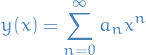
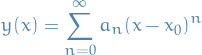
Frobenius method refers to the method where we assume the solution of a differential equation to be analytic, i.e. we can expand it as a power series:
Substituting this into the differential equation, we can quite often derive recurrence-relations by grouping powers of and solving for  .
.
Honours Differential Equations
Equations / Theorems
Reduction of order
Go-to way
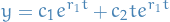
If we have some repeated roots of the characteristic equation , then the general solution is
where we've taken the linear combination of the "original" solution

and the one obtained from reduction of order
General
If we know a solution  to an ODE, we can reduce the order by 1, by assuming another solution
  of the form
where  is some arbitrary function which we can find from the linear system obtained from
  ,
,  and
and  . Solving this system gives us

i.e. we multiply our first solution with a first-order polynomial to obtain a second solution.
Integrating factor
Assume  to be a solution, then in a 2nd order homogeneous ODE we get the
Which means we can obtain a solution by simply solving the quadratic above.
This can also be performed for higher order homogeneous ODEs.
Repeated roots
What if we have a root of algebraic multiplicity greater than one?
If the algebraic multiplicity is 2, then we can use reduction of order and multiply the first solution for this root with the .
Factorization of higher order polynomials (Long division of polynomials)
Suppose we want to compute the following
- Divide the first highest order factor of the polynomial by the highest order factor of the divisor, i.e. divide
 by
by  , which gives
- Multiply the from the above through by the divisor
 , thus giving us
- We subtract this from the corresponding terms of the polynomial, i.e.

- Divide this remainder by the highest order term in of the divisor again, and repeating this process until we cannot divide by the highest order term of the divisor.
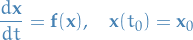
Existence and uniqueness theorem
Consider the IVP

where  ,
,  , and are continuous on an open interval
  that contains the point
  . There is exactly one solution
  of this problem, and the solution exists throughout the interval .
Exact differential equation
Let the functions  and
and  , where subscripts denote the partial derivatives, be continuous in the rectangular region
  . Then
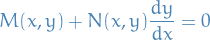
is an exact differential equation in if and only if
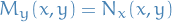
at each point of . That is, there exists a function  such that

if and only if  and
and  satisfy the equality above above.
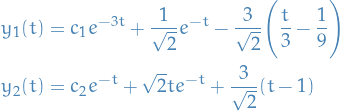
Variation of Parameters
Suppose we have the n-th order linear differential equation
Suppose we have found the solutions to the corresponding homogenous diff. eqn.
With the method of variation of parameters we seek a particular solution of the form
Since we have functions to determine we have to specify conditions.
One of these conditions is cleary that we need to satisfy the non-homongenous diff. eqn. above. Then the other conditions are chosen to make the computations as simple as possible.
Taking the first partial derivative wrt. of we get (using the product rule)
We can hardly expect it to be simpler to determine if we have to solve diff. eqns. of higher order than what we started out with; hence we try to surpress the terms that lead to higher derivatives of by imposing the following condition
which we can do since we're just looking for some arbitrary functions . The expression for then reduces to
Continuing this process for the derivatives we obtain our condtions:
giving us the expression for the m-th derivative of to be
Finally, imposing that has to satisfy the original non-homogenous diff. eqn. we take the derivative of and substitute back into the equation. Doing this, and grouping terms involving each of together with their derivatives, most of the terms drop out due to being a solution to the homogenous diff. eqn., yielding
Together with the previous conditons we end up with a system of linear equations
(note the at the end!).
The sufficient condition for the existence of a solution of the system of equations is that the determinant of coefficients is nonzero for each value of . However, this is guaranteed since form a fundamental set of solutions for the homogenous eqn.
In fact, using Cramers rule we can write the solution of the system of equations in the form
where is the determinant of obtained from by replacing the m-th column by . This gives us the particular solution
where is arbitrary.
Suppose you have a non-homogenous differential equation of the form

and we want to find the general solution, i.e. a lin. comb. of the solutions to the corresponding homogenous diff. eqn. and a particular solution. Suppose that we find the solution of the homogenous dif. eqn. to be
The idea in the method of variation of parameters is that we replace the constants  and
and  in the homogenous solution with functions
  and
and  which we want to produce solutions to the non-homogenous diff. eqn. that are independent to the solutions obtained for the homogenous diff. eqn.
Substituting 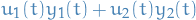 into the non-homogenous diff. eqn. we eventually get

which we can solve to obtain our general solution for the non-homogenous diff. eqn.
If the functions and are continuous on an open interval , and if the functions and are a fundamental set of solutions of the homogenous differential equation corresponding to the non-homogenous differential equation of the form
then a particular solution is

where is any conventional chosen point in . The general solution is

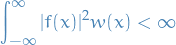
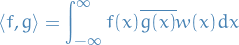
Parseval's Theorem
The square norm  of a periodic function with convergent Fourier series
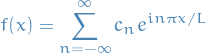
satisfies
![\begin{equation*}
\begin{split}
\langle f, f \rangle &= \int_{-L}^{L} |f(x)|^2 \ dx = 2L \sum_{n=-\infty}^{\infty} |c_n|^2 \\
&= L \Bigg[ \frac{|a_0|^2}{2} + \sum_{n=1}^{\infty} \Big( |a_n|^2 + |b_n|^2 \Big) \Bigg]
\end{split}
\end{equation*}](../../assets/latex/differential_equations_60061fb2aee1e71c45146c6c79502149abbfaceb.png)
By definition and linearity,
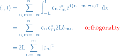
For the last equality, we just need to remember that
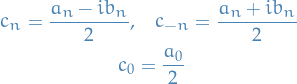
Indeed,
![\begin{equation*}
\begin{split}
2 L \sum_{n = -\infty}^{\infty} |c_n|^2 &= 2 L \Bigg[ |c_0|^2 + \sum_{n = 1}^{\infty} \Big( |c_n|^2 + |c_{-n}|^2 \Big) \Bigg] \\
&= 2 L \Bigg[ \frac{|a_0|^2}{4} + \sum_{n=1}^{\infty} \Bigg( \frac{|a_n|^2 + |b_n|^2}{4} + \frac{|a_n|^2 + |b_n|^2}{4} \Bigg) \Bigg] \\
&= L \Bigg[ \frac{|a_0|^2}{2} + \sum_{n=1}^{\infty} \Big( |a_n|^2 + |b_n|^2 \Big) \Bigg]
\end{split}
\end{equation*}](../../assets/latex/differential_equations_801f5f374d921cf944c5b8ccdf5a2cedf67a0524.png)
We also have a Parseval's Identity for Sturm-Liouville problems:
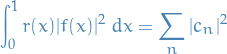
where the set  is determined as
and are the corresponding eigenfunctions of the SL-problem.
The proof is a simple use of the orthogonality of the eigenfunctions.
Binomial Theorem
Let be a real number and  a postive integer. Further, define
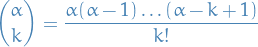
Then, if  ,
,
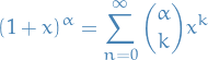
which converges for  .
.
This is due to the Mclaurin expansion (Taylor expansion about ).
Definitions
Words
- bifurication
- the appearance of a new solution at a certain parameter value
Wronskian
For a set of solutions 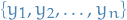 , we have
![\begin{equation*}
W[y_1, \dots, y_n] := \begin{vmatrix}
y_1 & y_2 & \dots & y_n \\
y_1' & y_2' & \dots & y_n' \\
\vdots & \vdots & \vdots & \vdots \\
y_1^{(n-1)} & y_2^{(n-1)} & \dots & y_n^{(n-1)}
\end{vmatrix}
\end{equation*}](../../assets/latex/differential_equations_1a6baed3e38084f4fd1a17f0dfda5f8b7c11d63d.png)
i.e. the Wronskian is just the determinant of the solutions to the ODE, which we can then use to tell whether or not the solutions are linearly independent, i.e. if ![$W[y_1, y_2, \dots, y_n] \ne 0$](../../assets/latex/differential_equations_547ccfe9d2e4c44ef5aeaacd2de3228bf5c66956.png) we have lin. indep. solutions and thus a unique solution for all initial conditions.
we have lin. indep. solutions and thus a unique solution for all initial conditions.
Why?
If you look at the Wronskian again, it's the determinant of the matrix representing the system of linear equations used to solve for a specific vector of initial conditions (if you set the matrix we're taking the determinant of above equal to some  which is the initial conditions).
The determinant of this system of linear equations then tells if it's possible to assign coefficients to these different solutions s.t. we can satisfy any initial conditions, or more specific, there exists a unique solution for each initial condition!
- if
![$W[y_1, \dots, y_n] \ne 0$](../../assets/latex/differential_equations_3a57da31ba61c1c6cf702ab6b5bc8604a2a07c84.png) then the system of linear equations is an invertible matrix, and thus we have a unique solution for each
then the system of linear equations is an invertible matrix, and thus we have a unique solution for each - if
![$W[y_1, \dots, y_n] = 0$](../../assets/latex/differential_equations_1fbe7b9a2ece91aa570a84531d403f60032dd01c.png) we do NOT have a unique solution for each initial condition
we do NOT have a unique solution for each initial condition
Thus we're providing an answer to the question: do the linear combination of  include all possible equations?
Properties
- If then
 \ne 0$](../../assets/latex/differential_equations_a3b2a960031335ca5954f9d40f84d17958339376.png) for all
for all ![$x \in [\alpha, \beta]$](../../assets/latex/differential_equations_1994f890f501056112a9489a992c228cca78a71b.png)
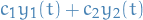
- Any solution can be written as a lin. comb. of any fundamental set of solutions

- The solutions form a fundamental set iff they are linearly independent
Proof of property 1
If  somewhere,
  everywhere for
Assume  at
at 
Consider
which can be written

with 
Hence,  such that (*) holds.
Thus, we can construct  which satisfies the ODE at
Proof of property 2
We want to show that  can satisfy any

Linearly independent →  and since
  , by property 1 we can solve it.
Homogenenous n-th order linear ODEs
![\begin{equation*}
L[y] = \frac{d^n y}{dx^n} + p_1(x) \frac{d^{n - 1} y}{dx^{n-1}} + \dots \ p_{n-1}(x) \frac{dy}{dx} + p_n(x) y = 0
\end{equation*}](../../assets/latex/differential_equations_ea2325c1a1b6bb3846562b386b302f58c2d9ea99.png)
Solutions  to homogeneous ODEs forms a vector space
Non-homogeneous n-th order linear ODEs
![\begin{equation*}
L[y] = \frac{d^n y}{dx^n} + p_1(x) \frac{d^{n - 1} y}{dx^{n-1}} + \dots \ p_{n-1}(x) \frac{dy}{dx} + p_n(x) y = g(x)
\end{equation*}](../../assets/latex/differential_equations_5a0eecfcf96a26ffbf2e45636847b1e2528d5834.png)
Solution
- Solve the corresponding homogeneous linear ODE
- Find special case solution for the non-homogeneous
- General solution is then the linear combination of these

 is some specific solution to the non-homogenous equation.
Power series
Laplace transform
An integral transform is a relation of the form
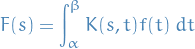
where  is a given function, called the kernel of the transformation, and the limits of integration and
  are also given.
Suppose that
- is piecewise continuous on the interval
 for any positive
  .
. 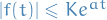 when
when  . In this inequality, , , and are real constants, and necessarily positive.
Then the Laplace transform of , denoted  or by
or by  , is defined
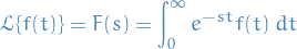
and exists for  .
.
Under these restrictions a function which increases faster than  is does not converge and thus the Laplace transform is not defined for this .
Properties
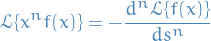
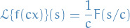
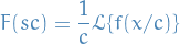
- Identities
Let
 , for
, for 
- Linear operator
The Laplace transform is a linear operator:

- Uniqueness of transform
We can use the Laplace transform to solve a differential equation, and by
- Inverse is linear operator
Frequently, a Laplace transform
is expressible as a sum of serveral terms

Suppose that
 . Then the function

has the Laplace transform
. By the uniqueness property stated previously, no other continuous function has the same transform. Thus

that is, the inverse Laplace transform is also a linear operator.

 and
and  for
for  :
:


Solution to IVP
Suppose that functions 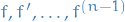 are continuous and that
  is piecewise continuous on any interval . Suppose further that

Then exists for  and is given by

We only prove it for the first derivative case, since this can then be expanded for the nth order derivative.
Consider the integral
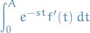
whose limit as  , if it exists, is the Laplace transform of .
Suppose is piecewise continuous, we can partition the interval and write the integral as follows

Integrating each term on the RHS by parts yields
![\begin{equation*}
\begin{split}
\int_0^A e^{-st} f'(t) \ dt =& e^{-st} f(t) \Big|_0^{t_1} + e^{-st} f(t) \Big|_{t_1}^{t_2} + \dots + e^{-st} f(t) \Big|_{k}^{A} \\
& + \Bigg[ \int_0^{t_1} e^{-st} f(t) \ dt + \int_{t_1}^{t_2} e^{-st} f(t) \ dt + \dots + \int_{t_k}^{A} e^{-st} f(t) \ dt \Bigg]
\end{split}
\end{equation*}](../../assets/latex/differential_equations_a449b0901801026f0aa88273456350b568ab6502.png)
since is continuous, the contributions of the integrated terms at  cancel, and we can combine the integrals into a single integral, again due to continuity:
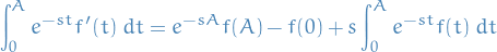
Now finally letting (since that's what we do in the Laplace tranform ) we note that
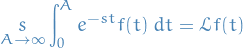
And since  , we have
 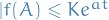 ; consequently

Finally giving us

Typical ones

Fourier Series
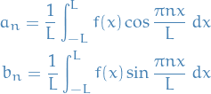
Given a periodic function with period  , it can be expressed as a Fourier series
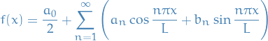
where the coefficients are given by
Suppose and  are piecewise continuous for
 ![$x \in [-L, L]$](../../assets/latex/differential_equations_671b6022d7b856a36a3a110821724082a4610022.png) .
.
Suppose is defined outside the interval so that it is periodic with period . Then the Fourier series of converges to where is continuous and to 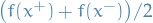 where is discontinuous.
Heavside function
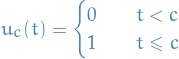
Which has a discontinuity at  .
.
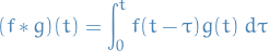
Convolution integral
If and are piecewise continuous functions on  then the convolution integral of and is,
Laplace transform

Phase plane
A phase plane is a visual display of certain characteristics of certain kinds of differential equations; a coodinate plane with axes being the values of the two state variables, e.g. .
It's a two-dimensional case of the general n-dimensional phase space .
Trajectory
A trajectory of a system
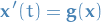
simply refers to a solution for some specific initial conditions , i.e.

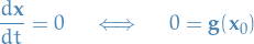
Critical points
Points corresponding to constant solutions or equilibrium solutions, of the following equation

are often called critical points.
That is, points such that
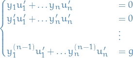
There always exists a coordinate transformation , such that
such that the new system
has an equilibrium solution or critical point at the origin.
Special differential equations / solutions
Legendre equation
The Legendre equation is given below:

We only need to consider  since if
  we can reparametrize the equation to be of the form above anyways.
In the case where we assume  , we note that for even
  becomes a terminating series, rather than an infinite series, and if is odd is a terminating series, i.e. in both cases we get a polynomial of order !
These polymomials corresponding to a solution of the Legendre equation for a specific integer we call a Legendre Polynomial, denoted  .
.
![\begin{equation*}
P_{\ell}(x) = \frac{1}{2^{\ell} \ell!} \frac{d^{\ell}}{dx^{\ell}} \Big[ (x^2 - 1)^{\ell} \Big]
\end{equation*}](../../assets/latex/differential_equations_940cb67f32f04309801cd7081d71273f5ab675ac.png)
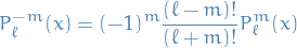
Or the general Legendre equation :
![\begin{equation*}
(1 - x^2) y'' - 2x y' + \Bigg[ \ell (\ell + 1) - \frac{m^2}{1 - x^2} \Bigg] y = 0
\end{equation*}](../../assets/latex/differential_equations_fc1168ae92c05fcb50130305913184fac581ff1c.png)
Which gives rise to the polynomials defined
where are the corresponding Legendre polynomial.
Moreover, using Rodrigues formula
If we let  we can use the relationship between
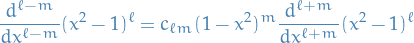
to obtain the coefficient
Series Solutions
The sum of the even terms is given by:

and the sum of the odd terms are given by:

TODO Legendre polynomials and Laplace equation using spherical coordinates
Van der Pol oscillator
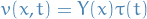
where is the position coordinate, which is a function of time , and is a scalar parameter indicating the nonlinearity and the strength of the damping.
Hermite polynomials
We are talking about the physicsts' Hermite polynomials given by
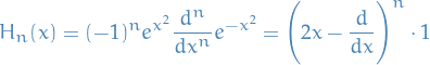
These are a orthonormal polynomial sequence, and they arise from the differential equation

These polynomials are orthogonal wrt. the weight function  , i.e. we have

Furthermore, the Hermite polynomials form an orthogonal basis of a the Hilbert space of functions satisfying
in which the inner product is given by the integral including the Gaussian inner product defined previously:
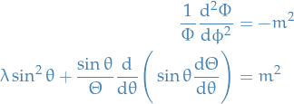
Spherical harmonics
In this section we're looking to tackle the spherical harmonics once and for all.
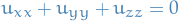
If we have a look at the Laplace equation in spherical coordinates, we have
If we then use separation of variables, and consider solutions of the form:

We get the following differential equations:
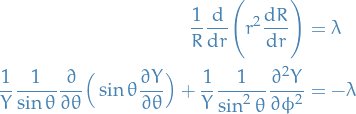
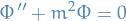
Further, assuming  , we can rewrite the second differential equation as
for some number .
Solving for
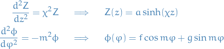
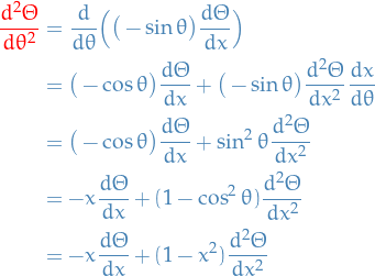
First we take a look at the differential equation involving ,
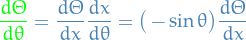
Which we can rewrite as
making the substitution

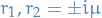
This is fine, since in spherical coordinates we have  , i.e.
  is always defined.
Thus,
Substituting back into the differential equation, we get
which has the general solution
where
solves
or rather,

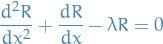
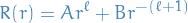
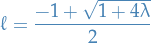
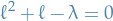
RECOGNIZE THIS YO?! How about trying to substitute this into the differential equation involving  ?
?
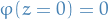
Solving for 
The differential equation with can be written
which has the solution

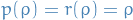
Further, we have the boundary condition  , which implies
  .
.
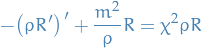
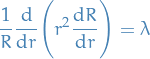
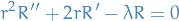
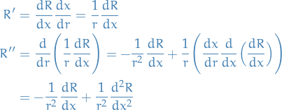
Solving for
We have the the ODE
which we can write out to get

Making the substitution  we have
And,
Substituting back into the ODE from above:
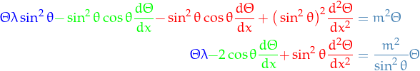
Observing that

We can write the above equation as
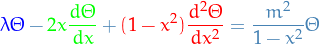
Whiiiich, we recognize as the general Legendre differential equation!
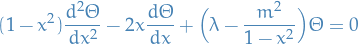
where we're only lacking the  , for which we have to turn to the differential equation involving
  .
.
With obtained from Solving for , we can rewrite the differential equation involving as

For which we know that the solutions are the corresponding associated Legendré polynomials

which are obtained by considering the series solution of the equation above, i.e. assuming:
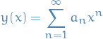
where is as above. Substituting into the differential equation above, and finding the recurrence-relation for we recover the Legendre polynomials mentioned above.
Bringing and together
Now, finally bringing this together with the solution obtained for , we have the spherical harmonics

where  is simply the normalization constant to such that the eigenfunctions form a basis, which turns out to be
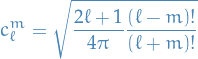
Thus, the final expression for the spherical harmonics is
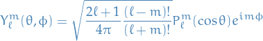
Combining everything
Finally, combining the radial solution and the spherical harmonics into the final expression for our solutions:

where we have set  to ensure regularity at
  , and not have the following occur:

Boundary conditions
- Establish that must be periodic (since we're working in spherical coordinates) whose period evenly divides
 , which implies and is a linear combination of
- Using what we observed in 1. and noting that
 is "regular" at the poles of the sphere, where
  , we have a boundary condition for (which is a Sturm-Liouville problem) forcing the parameter to be of the form
- Making the change of variables
 trnasforms this equation into the general Legendre equation, whose solution is a multiple of the associated Legendre Polynomial.
 Finally, the equation for
has solutions of the form
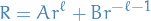
- If we want the solution to be "regular" throughout
 , we have .
When we say regular, we mean that the solution  has the property

Proper description
A priori is a complex number, BUT because must be a periodic function whose period evenly divides , is necessarily an integer and is a linear combination of the complex exponentials .
Further, the solution function is regular at the poles of the sphere, where . Imposing this regularity in the solution of the second equation at the boundary of the domain is a Sturm-Liouville problem that forces the parameter to be of the form

Furthermore, a change of variables transforms this equation into the (general) Legendre equation, whose solution is a multiple of the associated Legendre polynomial  .
.
Finally, the equation for has solutions of the form
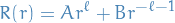
And if we require solution to be regular throughout forces .
Solutions
Here, the solution assumed to have the special form . For a given value of , there are  independent solutions of this form, one for each integer
  . These angular solutions are a product of trigonometric functions, here represented as a complex exponential, and associated Legendre polynomials:
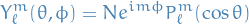
which fulfill

The general solution to the Laplace's equation in a ball centered at the origin is a linear combination of the spherical harmonic functions multiplied by the appropriate scale factor  ,
,
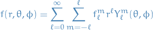
where the  are constants the factors
  are known as solid harmonics.
Q & A
DONE Why do we actually require the to be an integer?
In solving for we observe that
Thus, if we require to be true, then we need to "go full circle" every  , hence .
If it does NOT go full circle, then it would be discontinuous.
DONE We have TWO explanations for why we need , which one is true?
- Question
Here we state that
has to be "because it's a Sturm-Liouville problem". I don't understand why it being a Sturm-Liouville problem necessarily imposes this restriction.
Ah! Maybe it's because Sturm-Liouville problems require the limiting behavior of the boundary conditions to satisfy Lagrange's identity being zero!
While here, we simply solve the differential equation involving
, and just falls out from this solution, and as far as I can tell, we're not actually saying anything about the boundary conditions in this case.
- Answer
From what I can understand, the eigenvalue
simply falls out from as we found, and being of this form does not seem to be related in any way to boundary conditions.
What is related to the boundary conditions, the fact that
is an integer.
What is related to the b
Bessel equation
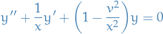
This can be solved using Frobenius method.
In the case where  , we end up with the Bessel function of the 1st kind :
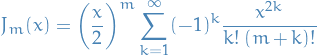
And the Bessel function of the 2nd kind :
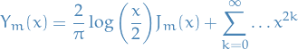
Thus, the general solution will be the linear combination:

Where we have the following limiting behavior:
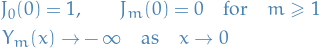
Note: Quite often we want the solution to be "regular" / nicely behaved as  , thus we often end up setting
  in the expression for
  .
.
Problems
10.2 Fourier Series
Ex. 10.2.1
Assume that there is a Fourier series converging to the function defined by
with the property that
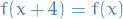
i.e. it's periodic with a period of 4.
Find the components of the Fourier series.
Solution
See p. 601 in (Boyce, 2013) for the full solution.
10.5 Separation of variables; Heat conduction in a Rod
Find the solution of the heat conduction problem
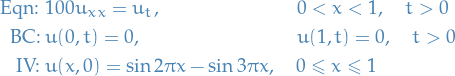 1
1
Solution

We suppose

And the boundary conditions are satisfied by

First we note that with above we get the following

which gives
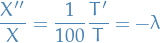
for some constant , which gives us the system
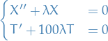
The solution to the first equation simply gives us

Considering the boundary conditions, we get
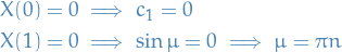
thus we get the eigenfunctions and eigenvalues for  :
:

Substituting these eigenvalues into the differential equation with :
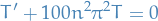
which can be solved by use of integrating factors, thus
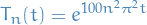
Finally, combining both into the eigenfunctions for the entire solution 

Which gives us the general solution:
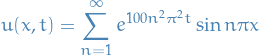
and solving for the coefficients using the initial conditions, i.e. when

Hence the final solution is
