Linear Algebra
Table of Contents
Definitions
Ill-conditoned matrix
A matrix  is ill-conditioned if small changes in its entries can produce large
changes in the olutisns to
is ill-conditioned if small changes in its entries can produce large
changes in the olutisns to  . If small changes in the entries
of produce small changes in the solutions to , then
is called well-conditioned.
. If small changes in the entries
of produce small changes in the solutions to , then
is called well-conditioned.
Singular values
For any  matrix , the
 is symmetric and thus orthogonally diagonalizable
by the Spectral Theorem.
is symmetric and thus orthogonally diagonalizable
by the Spectral Theorem.
The eigenvalues of are real and non-negative. Therefore,
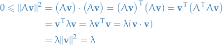 1
1
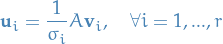
where  is a unit eigenvector of . Hence, we can take the square root
of all these eigenvalues, and define what we call singular values:
is a unit eigenvector of . Hence, we can take the square root
of all these eigenvalues, and define what we call singular values:
If is an matrx, the singular values of are the square roots
of the eigenvalues of and are denoted  .
.

By convention we order the singular values s.t.  .
.
Cholesky decomposition
The Cholesky decomposition or Cholesky factorization is a decomposition of a Hermitian positive-definite matrix into a product of lower triangular matrix and it's conjugate transpose:

where  is lower-triangular.
Every Hermitian matrix has a unique Cholesky decomposition.
A real Cholesky factor is unique up to sign of the columns.
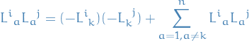
Suppose is Cholesky factor of some matrix. The matrix components are then given by
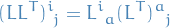
So by scaling the k-th column by -1 we get
So it ain't no matter:)
Sidenote: summing all the way to  is redundant because all indices larger than
  vanishes.
Theorems
Spectral Theorem
Let be an real matrix. Then is symmetric iff it is orthogonally diagonalizable.
Singular Value Decomposition
Let be an matrix with singular values  and
and
 . Then there exists:
 orthogonal matrix
- orthogonal matrix

- "diagonal" matrix
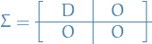 , where
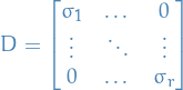
such that:

See page 615 of "Linear Algebra: A Modern Introduction" :)
Constructing V
To construct the orthogonal matrix , we first find an orthonormal basis  for
for  consisting of eigenvectors of the symmetric matrix . Then
![\begin{equation*}
V = [ \mathbf{v}_1 \cdots \mathbf{v}_n ]
\end{equation*}](../../assets/latex/linear_algebra_379644cea68ba33c9ab9c11aa9187e8fa8d7bab8.png)
is an orthogonal matrix.
Constructing U
For the orthogonal matrix , we first note that 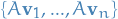 is an orthogonal set of vectors
in
is an orthogonal set of vectors
in  (we're NOT saying they form a basis in !). To see this, suppose that
  is a
eigenvector of corresponding to the eigenvalue
is a
eigenvector of corresponding to the eigenvalue  . Then, for
  , we have
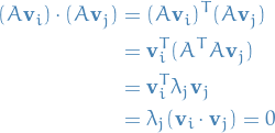
since the eigenvectors are orthogonal.
Since  we can normalize
  by
by
This guarantees that  is a orthonormal set in ,
but if
is a orthonormal set in ,
but if  it's not a basis. In this case, we extend
to an orthonormal basis
it's not a basis. In this case, we extend
to an orthonormal basis  for by some
technique, e.g. the Gram-Schmidt Process, giving us
for by some
technique, e.g. the Gram-Schmidt Process, giving us
![\begin{equation*}
U = [ \mathbf{u}_1 \cdots \mathbf{u}_m ]
\end{equation*}](../../assets/latex/linear_algebra_8bd4e5a916a48fdd78852a680c82aaeb5f042556.png)
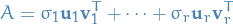
Outer Product Form of the SVD
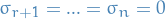
Let be an matrix with singular values
and  , then
Geometric insight into the effect of matrix transformations
Let be an matrix with rank  . Then the image of the unit sphere in
under the matrix transformation that maps
. Then the image of the unit sphere in
under the matrix transformation that maps  to
to  is
is
- the surface of a an ellipsoid in if

- a solid ellipsoid in if

We have  with
with 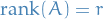 . Then

Let  (i.e. unit vector = surface of unit sphere) in
  .
is orthogonal, thus
.
is orthogonal, thus  is orthogonal and then
  is a unit vector too.
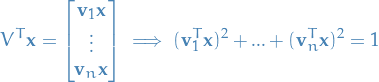
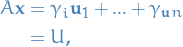
From the Outer Product Form we have:
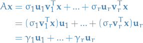
where we are letting  denote the scalar
  .
.
(1) If  , then we must have
  and
and
Since is orthogonal, we have  , thus
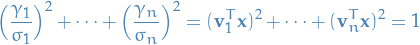
which shows that the vectors form the surface of an ellipsoid in !
(2) If , swapping equality with inequality (but performing the same steps):
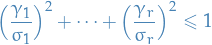
where the inequality corresponds to a solid ellipsoid in !
Furthermore, we can view the each of the matrix transformations of the SVD separately:
- is an orthogonal matrix, thus it maps the unit sphere onto itself (but in a different basis)
- matrix
 first collapses to
  dimensions of the unit sphere,
leaving a unit sphere of dimensions, and then "distorts" into an ellipsoid
dimensions of the unit sphere,
leaving a unit sphere of dimensions, and then "distorts" into an ellipsoid - is orthogonal, aligning the axes of this ellipsoid with the orthonormal basis vectors $ 1, …, r$ in
Least squares solution for dependent column-vectors
The least squares problem has a unique least squares solution  of minimal
length that is given by:
of minimal
length that is given by:

See page 627 of "Linear Algebra: A Modern Introduction" :)
Determinant
Trace is the sum of the eigenvalues
Let  be a matrix, then
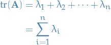
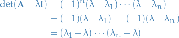
We start with the characteristic equation

We then notice that

which can be seen by expanding the determinant along the diagonal:
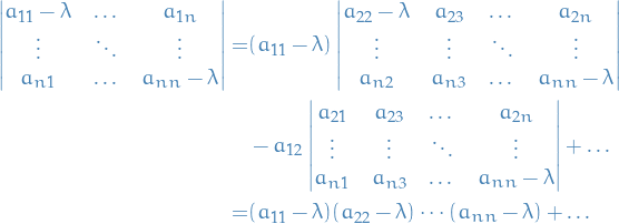
Here we see that the only "sub-determinant" which contains a factor of  is going to be the very first one which is multiplied by
  , since each of the other "sub-determinants" will not have a coefficient with
  , and it will not contain
  , hence at most contain a factor of
  .
.
Further, since

we observe that 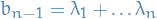 , which we also know to be the
  from above, i.e.

as wanted.
Determinant is the product of the eigenvalues
Let be a matrix, then
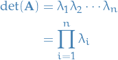
Let be a matrix. Then

defines the characteristic equation, which as the eigenvalues as its roots, therefore
Since is just a variable, we let  and get

as wanted.
Cramers Rule
Consider the system of linear equations represented by unknowns; in matrix form

where  has nonzero determinant, then
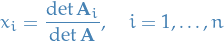
where  is the matrix formed by replacing the i-th column of by the column vector
  .
.
The reason why we can think of OLS as projection
The proof of the following theorem is really important in my opinion, as it provides a "intuitive" way of viewing least-squares approximations.
The Best Approximation Theorem says the following:
If  is a finite-dimensional subspace of an inner product space and if
is a vector in , then
is a finite-dimensional subspace of an inner product space and if
is a vector in , then  is the best approximation to in .
Let  be a vector in different from .
Then
be a vector in different from .
Then  is also in , so
  is orthogonal to .
Pythagoras' Theorem now implies that

But  , so
, so

i.e.  and thus that is the best approximation.
Distance and Approximation
Applications
Function-approximation
Given a continunous function  on an interval
 ![$[a, b]$](../../assets/latex/linear_algebra_c9a1e8df376ecb942b106e02d3e6d1b417da2600.png) and a subspace of
and a subspace of ![$\mathcal{C}[a, b]$](../../assets/latex/linear_algebra_522cb05ba5d1c97eeff01816075d0fba81fe6149.png) ,
find the function "closest" to in .
,
find the function "closest" to in .
- denotes the space of all continuous functions defined on the domain
- is a subspace of
Problem is analogous to least squares fitting of data points, except we have infinitely
many data points - namely, the points in the graph of the function .
What should "approximate" mean in this context? Best Approximation Theorem has the answer!
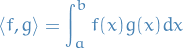
The given function lives in the vector space of continuous functions on
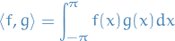
the interval . This is an inner product space, with inner product:
If is finite-dimensional subspace of , then the best approximation to
in is given by the projection of onto .
Furthermore, if  is an orthogonal basis for , then

The error from this approximation is just
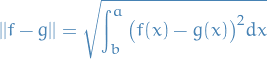
and is often called the root mean square error. For functions we can think of this as the area between the graphs.
Fourier approximation
A function of the form

is called a trigonometric polynomial.
Restricting our attention to the space of continuous functions
on the interval ![$[- \pi, \pi ]$](../../assets/latex/linear_algebra_dab0d85594f921c74674fee47916c345db89fbca.png) , i.e.
, i.e. ![$\mathcal{C}[-\pi, \pi]$](../../assets/latex/linear_algebra_40ef2fba60d64669dd52c0be6c03a02d90ecf040.png) , with the inner product
, with the inner product
and since the trigonometric polynomials are linear combinations of the set

the best approximation to a function in by
trigonometric polynomials of order is therefore  ,
where
,
where  . It turns out that
  is an orthogonal set,
hence a basis for .
is an orthogonal set,
hence a basis for .
The approximation to using trigonometric polynomials is called the
n-th order Fourier approximation to on ![$[-\pi, \pi]$](../../assets/latex/linear_algebra_aa62fe947306d8dbe0a258bbfdc3c84c03ffff2f.png) , with the coefficients
are known as Fourier coefficients of .
, with the coefficients
are known as Fourier coefficients of .
Rayleigh principle
A lot of the stuff here I got from these lecture notes.
Notation
 denotes the Rayleigh coefficient of some Herimitian / real symmetric matrix
  is the diagonal matrix with entries being eigenvalues of
 - Eigenvalues are ordered as
 is the orthogonal matrix with eigenvectors of as columns
 , thus
Definition
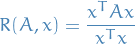
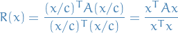
For a given complex Hermitian matrix and non-zero vector  , the Rayleigh quotient is defined as:
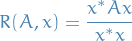
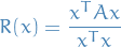
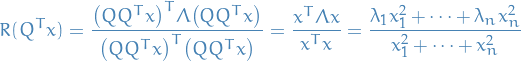
In the case of , and is symmetric, then
Further, in general,
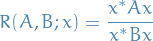
is the generalized Rayleigh quotient, where  is a positive-definite Herimitian matrix.
The generalized Rayleigh quotient can be reduced to  through the transformation

where  is the Cholesky decomposition of the Hermitian positive-definite matrix .
Minimization
Personal explanation
At the maximum we must have
But observe that for whatever  we have here, we have
i.e. it's invariant to scaling.
Further, since is symmetric, we have the diagonalization

which means that if we let

for some  , we get

where we've applied the constraint 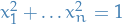 , which we can since again, invariant under scaling.
Therefore, we're left with the following optimization problem:
Since we assume that , we clearly obtain the minima when
Hence,

where  denotes the corresponding eigenvector.
Now suppose we'd like to find the minima, which is NOT in the space spanned by the first eigenvector, then we only consider the subspace

Thus, the optimization problem is
Finally, observe that  , hence
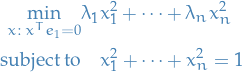
And the subspace  is just all
 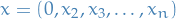 , giving us

And if we just keep going, heyooo, we get all our eigenvalues and eigenvectors!
Stuff
We're going to assume is real.
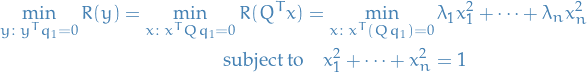
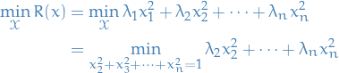
Our objective is:

Observe the following:
- Objective is invariant to scaling, since we'd be scaling the denominator too
- is by assumption symmetric: all real eigenvalues
Thus, we have
Further,

Hence,
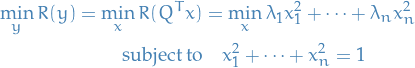
Thus, by letting , we get
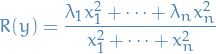
Since this quotient is invariant under scaling, we frame it as follows:

Implying that ![$R(y) \in [\lambda_1, \lambda_n]$](../../assets/latex/linear_algebra_8dcc526f9d7daac89b97f0e234be47ae85de1bf8.png) (seen from
(seen from  and
and  ) since we assume the eigenvalues to be ordered.
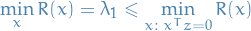
Hence, we have proved what's called the Rayleigh Principle:
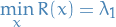
where  is the smallest eigenvalue of .
Planar Slices
Suppose we'd like to find the answer to the following:

i.e. minimizing the Rayleigh quotient over some hyperplane defined by  .
.
This minimum is bounded blow as follows:
Further, we can obtain an upper bound for this by considering  again:

By scaling we can assume 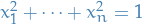 , giving us the optimization problem
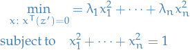
There is at least one vector of the form

If  , then the above translates to

assuming  (does not satisfy second constraint), then the first constraint can be represented as:
which is just a line through the origin. The second constraint is the unit-circle. Thus, there are only two points where both these constraints are satisfied (a line crosses the circle in two places). Let  be one of these points of intersection, then

Which means we have bounded the minimum of on the hyperplane ! This becomes incredibly useful when have a look at Minimax Principle for the Second Smallest Eigenvalue.
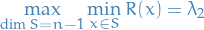
Minimax Principle for the Second Smallest Eigenvalue
This is a slighly different way of viewing finding the second eigenvalue, and poses the "answer" in a frame where we might have asked the following question:
"Can we obtain  without finding ?"
And ends with the answer:
which is very useful computationally, as we can alternate between miniziming and maximizing to obtain .
What if we could attain the maximum in this equation such that we would know that "maximizing in the hyperplane , where minimizes , gives us the second smallest eigenvalue !
Or equivalently, the minimum in the restricted hyperplane is given by !
Thus, if we can force somehow force  and
and  , then we would get a upper bound for this. If we had
  then the only solutions to this would be:

To show that  , we only consider solutions for where
  , i.e. let

Which is clearly attained when  and
and  , since
Hence,
Thus we've shown that min-maxing over some function is equivalent of finding the second smallest eigenvalue!
Since means that lies in the orthogonal complement of  , which is an (n-1)-dimensional subspace. Thus, we may rewrite the above as
In fact, it turns out this works for general  :
:
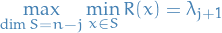
All this means that if we want to find some vector which minimizes the Rayleigh quotient, then we simply compute the eigenvalues of and look for the corresponding eigenvector, giving us the solution!