Calculus
Table of Contents
Calculus
Definitions
Norm / mesh of partition
The norm ( or mesh ) of the partition

is the length of the longest of these subintervals:

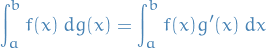
Riemann-Stieltjes integral
The Riemann-Stieltjes integral of a real-valued function  of a real variable with respect to a real function
  is denoted by
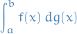
and defined to be the limit, as the norm of the partition

of the interval ![$[a, b]$](../../assets/latex/calculus_c9a1e8df376ecb942b106e02d3e6d1b417da2600.png) approaches zero, of the approximating sum
approaches zero, of the approximating sum
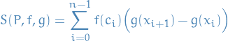
where  is in the i-th subinterval
 ![$[x_i, x_{i + 1}]$](../../assets/latex/calculus_223edbe88a9c512c258f555a18a9343c0cab5b28.png) . The two functions and are respectively called the integrand and the integrator.
. The two functions and are respectively called the integrand and the integrator.
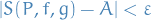
The "limit" is understood to be a number  (value of the Riemann-Stieltjes integral) such that for every
  there exists a
  s.t. every partition
  with
with 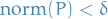 , and for every choice of points in ,
Comparison to Riemann integral
The Riemann integral for the case used in the definition above we have
Now, what's the difference between this and the Riemann-Stieltjes integral? The main point is that the Riemann-Stieltjes integral allow us to integrate wrt. the function  itself rather than to
  and then wrt.
  . In this way it extends the Riemann integral and is slightly more "general".
Equations / Theorems
Fundamental Theorem of Calculus
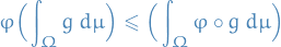
Jensen's Inequality
Let  be a probability space, i.e.
  , where
 is the set under consideration
 is a measure
- $A a sigma-algebra of
Then if
- is real-valued function that is -integrable
 is a convex function on the real line
we have:
TODO Proof
Vector calculus
Definitions
Conservative vector field
A conservative vector field is a vector field that is the gradient of some function, know in this context as a scalar potential.
Conservative vector fields have the property that a line integral is path independent , i.e. the choice of any path between two points does not change the value of the line integral.
Equations / Theorems
(Gauss') Divergence Theorem
"Integral definition"
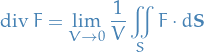
From what I can tell, this looks like the "approximation" near some point which can be arrived at from the Divergence Theorem using Stokes' Theorem. See this section for what I'm talking about.
Multivariate Taylor Expansion
![\begin{equation*}
f(\mathbf{x}) = f(\mathbf{a}) + \Big[(\mathbf{x} - \mathbf{a}) \cdot \Big( \boldsymbol{\nabla} \cdot f(\mathbf{x}) \Big) \Big] + \Big[ (\mathbf{x} - \mathbf{a}) \cdot \Big( H(\mathbf{x}) \cdot (\mathbf{x} - \mathbf{a}) \Big) \Big] + ...
\end{equation*}](../../assets/latex/calculus_2f0514f9f452d00fe687d9cfed66493c553625f6.png)
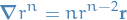
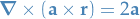
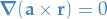
Vector field identities


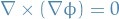
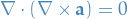

Elementary identities


Essential Calculus: Early Transcendentals
11 Vector Calculus
11.6 Directional Derivatives and the Gradient Vector
Directional Derivative
Finding the derivative of some function at some point  in the direction of some arbitrary unit vector
  .
.
 1
1
Which expresses the directional derivative in the direction of
as the scalar projection of the gradient vector onto .
- Maximizing the Directional Derivative
Suppose
is a differentiable function of two or three variables.
The maximum value of the directional derivative  is
is
 and it occurs when has the same direction as
the gradient vector
and it occurs when has the same direction as
the gradient vector  .
.

Which is simply maximized when
 , i.e. has the same direction as
  .
.
This just says that
has it's maximum change in the
direction of .
If you're at some point , and what the direction to move
for maximum change in , move in the direction of .
Tangent Planes to Level Surfaces
Let:
 is a surface with equation
  ,
i.e. it is a level surface of a function
,
i.e. it is a level surface of a function 
 be a point on
  be any curve that lies on the surface and pass through the point ,
i.e.
be any curve that lies on the surface and pass through the point ,
i.e.  where
where 
Then any point  must satisfy the equation of , that is:
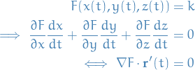
Which says that the gradient vector  of is orthogonal to the
gradient of any curve lying on that passes through .
Furthermore, this defines the a plane with the normal vector
and so we have a rather general definition of a tangent plane.
of is orthogonal to the
gradient of any curve lying on that passes through .
Furthermore, this defines the a plane with the normal vector
and so we have a rather general definition of a tangent plane.
This makes sense intuitively, because as we move away from the point
while staying on the level surface , the value of does not change.
That's the entire point of a level surface:  for some
  .
And the direction of maximum increase is then orthogonal to the level surface .
.
And the direction of maximum increase is then orthogonal to the level surface .
Notice where this comes in? Gradient descent. If we instead move
the opposite of the gradient, i.e. orthogonal to the level surface but
in the "negative" direction, we got ourselves the entire premise of GD.
11.8 Lagrange Multipliers
Overview
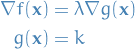
Goal is to find extreme values of  subject to the constraint
  . In other words, we seek the extreme values of when the point
  is restriced to lie on the level curve .
To maximize wrt.  is then to find the largest value
  such that the level curve
  intersects . This happens when and have the same tangent line . Otherwise, the value of could be increased further. This means that the normal lines at the point are parallel !

Algorithm
To find the maximum and minimum values of subject to the constraint [assuming that these extreme values exist and  on the surface ]:
a) Find all values of and  , s.t.:
b) Evaluate at all points that result from step (a). The largest of these values is the maximum value of : the smallest is the minimum value of .
13 Vector Calculus
Notation
- denotes a curve
 defines the path of the curve
  denotes the region enclosed by the curve
 - positive orientation of a simple closed curve refers to a single counterclockwise traversal of , i.e. the region is always on the left as the point traverses
13.4 Green's Theorem
This theorem gives us a neat "trick" to compute integrals for certain types of closed surfaces.
Let be a positively oriented, piecewise-smooth, single closed curve in the plane and let be the region bounded by . If and  have continuous partial derivatives on an open region that contains , then
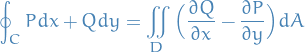
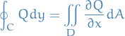
Notice that we have a proof if we can show that
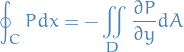
and
We write the region as:

where  and
and  are continuous functions.
Then,
![\begin{equation*}
\iint_D \frac{\partial P}{\partial y} \ dA = \int_a^b \int_{g_1(x)}^{g_2(x)} \frac{\partial P}{\partial y}(x, y) \ dy\ dx = \int_a^b [P(x, g_2(x)) - P(x, g_1(x))] \ dx
\end{equation*}](../../assets/latex/calculus_a8eccf2adce74e96133271c41fa775455823936f.png)
where the last step follows from the Fundamental Theorem of Calculus.
If the entire curve is smooth, we got our result. If it's only piecewise smooth, we then treat the curve as a union of piecewise smooth curves, and compute the integral for each of these piecewise curves making up .
Note that when computing this for the piecewise case, we need to make sure that we choose the correct sign for each of the integrals, i.e. sign s.t. that positive means enclosed surface is on the left.
Green's Theorem can also be extended to include surfaces with holes , i.e. regions which are NOT simply-connected .
This is done by splitting regions in such a way that we instead end up with multiple simply-connected surfaces.
See p. 787 in the book.
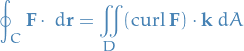
Vector forms
The following expresses Green's Theorem as the line integral of the tangential component of  along as the double integral of the vertical component of
  over the region D enclosed by .
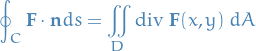
The other following expresses Green's Theorem as the line integral of the normal component of along is equal to the double integral of the divergence of over the region enclosed by .
13.5 Curl and Divergence
Curl
If  is a vector field on
  and the partial derivatives of , , and
  all exist, then the curl of is the vector field on defined by

- Why the name "curl"?
- Curl vecto is associated with rotations
- Another occus when represents the velocity field in fluid flow. Particles near
 in the fluid tend to rotate about the axis that points in the direction of
  and the length of this curl vector is a measure of how quickly the particles move around the axis.
Divergence
If is a vector field on and , , and have continuous second-order partial derivatives, then

- Why the name "divergence"?
Again, in the context of fluid flow .
If
 is the velocity field of a fluid, then
  represents the net rate of change (wrt. time) of the mass of the fluid flowing from point per unit volume.
In other words,
 measures the tendency of the fluid to diverge from the point .
If
 , then is said to be incompressible.
13.7 Surface Integrals
If is a continuous vector field defined on an oriented surface with a unit normal vector  , then the surface integral of over is
This integral is also called the flux of across .
And since:
we can also a surface integral:
Applications in Physics
- Notation
 fluid density at
  velocity field
- is surface the fluid is flowing through
- Fluid flow
We can approximate the mass of fluid crossing a segment of the surface,
 , in the direction of the normal per unit time by the quantity:
where
 is the area of the surface-segment .
Then by definition of a surface integral, summing these elements and taking the limit we get the rate of flow through the surface
as:
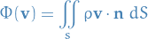
Also known as the flux.
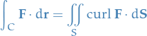
Stoke's Theorem
Let be an oriented piecewise-smooth surface that is bounded by a simple, closed, piecewise-smooth boundary curve with positive orientation. Let be a vector field whose components have continuous partial derivatives on an open region in that contains . Then
The book says I'm not smart enough to know yet. Some day…
Green's Theorem is a special case of Stoke's Theorem.
Shedding light on the curl of a vector field
Using Stoke's Theorem we can shed some more light on .
Suppose that is an oriented closed curve and  represents the velocity field in fluid flow. Consider the line integral
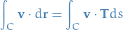
and recall that  is the component of in the direction of the unit tangent vector
  .
.
This means that the closer the direction of is to the direction of , the larger the value of . Thus  is a measure of the tendency of the fluid to move around and is called the circulation of around .
Now let  be a point in the fluid and let
  be a small disk with radius
  and center
  . Then
  for all points on becuase is continuous.
Thus, by Stokes' Theorem, we get the following approximation to the circulation around the boundary circle  :
:
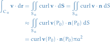
This approximation becomes better as  and we have
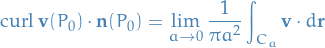
Hence, we have a relationship between the curl and the circulation, where we can view the  as a measure of the rotating effect of the fluid about the axis .
The curling effect is greatest about the axis parallel to  .
.
13.9 The Divergence Theorem
Let  be a simple solid region and let be the boundary surface of , given with positive (outward) orientation. Let be a vector field whose component functions have continuous partial derivatives on an open region that contains . Then
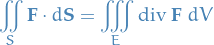
Thus the Divergence Theorem states that, under the given conditions, the flux of across the boundary surface of is equal to the triple integral of the divergence of over .