Functional Analysis
Table of Contents
Notation
 represents the Hilbert space over
Definitions
Bounded operator
We say a linear operator  is bounded if

If  and
and  are normed spaces, a linear map
  is bounded if

If  is bounded, then the supremum above is called the operator norm of , denoted
  .
.
Let be a normed space and be a Banach space.
Suppose  is a dense subspace of and
  is a bounded linear operator.
Then there exists a unique bounded linear map  such that

Furthermore,

Theorems
Riesz representation theorem
Notation
 denotes a Hilbert space
Theorem
This theorem establishes an important connection between a Hilbert space and its continuous dual space.
If the underlying field is  , then the Hilbert space is isometrically isomorphic to its dual space; if it's , then the Hilbert space is isometrically anti-isomorphic to the dual space.
Let be the Hilbert space, and  denote its dual space, consisting of all continous linear functionals from into the field or .
If  , then the functional
  is defined by:

then  .
.
The Riesz representation theorem states that every element of can be written uniquely in this form.
Given any continuous functional  , the corresponding element
  can be constructed uniquely by

where  is an orthonormal basis of , and the value
  does not vary by choice of basis.
Theorem: The mapping  defined by
  is an isometric (anti-) isomorphism, meaning that:
 is bijective
- The norms of
 and agree:
- is additive:

- If the base field is , then
 for
for 
- If the base field is , then
 for
for 
In the mathematical treatment of quantum mechanics, the theorem can be seen as a justification for the popular bra-ket notation. The theorem says that, every bra  has a corresponding ket
  , and the latter is unique.
When we say the dual space is continuous we mean that the linear operator acting on the functions (elements) in the Hilbert space
If  is a bounded linear functional, then there exists a unique
  such that

Furthermore, the operator norm of  as a linear functional is equal to the norm of
  as an element of .
The operator norm is defined as

Mercer's Theorem
Let ![$K: [a, b]^2 \to \mathbb{R}$](../../assets/latex/functional_analysis_9094fa2e92b0f7404e1360129684d05a5019f3c5.png) be a symmetric continuous function, often called a kernel.
be a symmetric continuous function, often called a kernel.
 is said to be non-negative definite (or positive semi-definite) if and only if
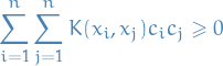
for all fininte sequences of points ![$x_1, \dots, x_n \in [a, b]$](../../assets/latex/functional_analysis_df408ebd5b590a92452fc6df4e55a0f880cc7ffc.png) and all choices of real numbers
and all choices of real numbers  .
.
We associate with a linear operator ![$T_K: L^2([a, b]) \to L^2([a, b])$](../../assets/latex/functional_analysis_5f9dfc4f9e9bcce9ac9d7c164cb268f6a8bc8c39.png) by
by
![\begin{equation*}
\big( T_K \varphi \big) (x) = \int_{a}^{b} K(x, s) \varphi(s) \ ds, \quad \varpih \in L^2([a, b])
\end{equation*}](../../assets/latex/functional_analysis_bc560a42951e0bd2cc0362cf49cbd1f028dcc30b.png)
The theorem then states that there is an orthonormal basis of ![$L^2([a, b])$](../../assets/latex/functional_analysis_46dd0ac7af731cb49a65fdba69a9f752782dd5f8.png) consisting for eigenfunctions of
consisting for eigenfunctions of  such that the corresponding sequence of eigenvalues
  is nonnegative.
The eigenfunctions corresponding to non-zero eigenvalues are continuous on ![$[,a b]$](../../assets/latex/functional_analysis_6be04418b084a48c01f8efb12c1e5320b79a368e.png) and has the representation
and has the representation
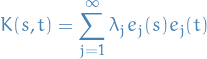
where the convergence is absolute and uniform.
There are alos more general versions of Mercer's thm which establishes the same result for measurable kernels, i.e.  on any compact Hausdorff space
  .
.
Generalized functions / distributions
Notation
 be a vector space over
  be its dual space
 be the vector space
  of functions
  with
with Stuff
- 'singular functions' occur as a rule only in intermediate stages of solut
Given a 'singular function' we know the result of its integration against a "good" function
 :
:
We say the sequence  with
with  converges to zero if
![\begin{equation*}
\varphi_n(x) = 0, \quad \forall x \notin I = [a, b], \forall n \in \mathbb{N}
\end{equation*}](../../assets/latex/functional_analysis_fa04ec7745bf944ecb8a44ba4482fde401f87e55.png)
i.e.  has bounded support, and and its derivatives converges uniformly to zero.
We say that the linear function  is continuous if

The set of continuous linear functionals is denoted  and its elements are called distributions or generalized functions.
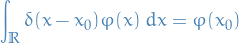
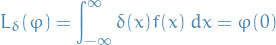
An example is the Dirac delta function  defined by
We can then define scalar multiplication over by functions  , then if
  and
and  , then

Since we can add distributions, we can construct linear combinations

of distributions with coefficients in the ring of  functions. Hence we have a module over
  !
!