Conditional Random Fields (CRFs)
Table of Contents
Overview
- Graphical model
- Is a discriminative model => attempts to directly model

Graphical models
Distributions over very many variables can often be represented as a product of local functions that depend on a much smaller subset of variables.
Undirected models
Notation
 is a set of rvs. that we target
 takes outcomes from the (continuous or discrete) set
 is an arbitrary assignment to
  denotes value assigned to
  by
by  is summation over all possible combinations of where
 is factor where
  is an index in
  ,
,  being the number of factors
 is a indicator variable, having value
  if
if  and
and  otherwise
 for some rvs.
  denotes the neighbors of in some graph
 usually denotes indices for rvs. of some graph
  usually denotes the indices for factors of some graph
Factors
- Believe probability distribution
 can be represented as a product of
factors
can be represented as a product of
factors - Each factor depends only on a subset
 of the variables
 - Non-negative scalar which can be thought of a compatibility measure between
the values

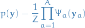
Formally, given a collections of subs  of , an unidirected graphical model
is the set of all distributions that can be written as
of , an unidirected graphical model
is the set of all distributions that can be written as
 1
1
for any choice of factors  that have
  for all .
We use the term random field to refer to a particular distribution among those defined by a unidirected graphical model.
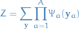
The constant  is the normalization factor (also referred to as the
parition function) that ensures the distribution sums to .
is the normalization factor (also referred to as the
parition function) that ensures the distribution sums to .
 2
2
Notice that the summation in is over the exponentially many possible assignments .
Factor graph
A factor graph is biparite graph  , i.e. a graph with
two disjoint sets of nodes
, i.e. a graph with
two disjoint sets of nodes  and
and  :
:
 indexes the rvs. in the model
- indexes the factors
By this representation, we mean that if a variable node for  is connected to a
factor node
is connected to a
factor node  for
for  then is one of the arguments of .
Markov network
A Markov network represents the conditional independence relationships
in a multivariate distribution, and is a graph over random variables only.
That is; is a graph over integers (rv. indices) .
A distribution is Markov with respect to if it satisfies the local
Markov property: for any two variables  , the variable
is independent of
, the variable
is independent of  conditioned on its neighbors,
  . Intuitively,
this means that contains all the information that is useful for
predicting
. Intuitively,
this means that contains all the information that is useful for
predicting
An issue with a Markov network is that it is ambigious, i.e. "not descriptive enough" from the factorization persepective. If you have a look at the figure below you can see an example of what we're talking about.
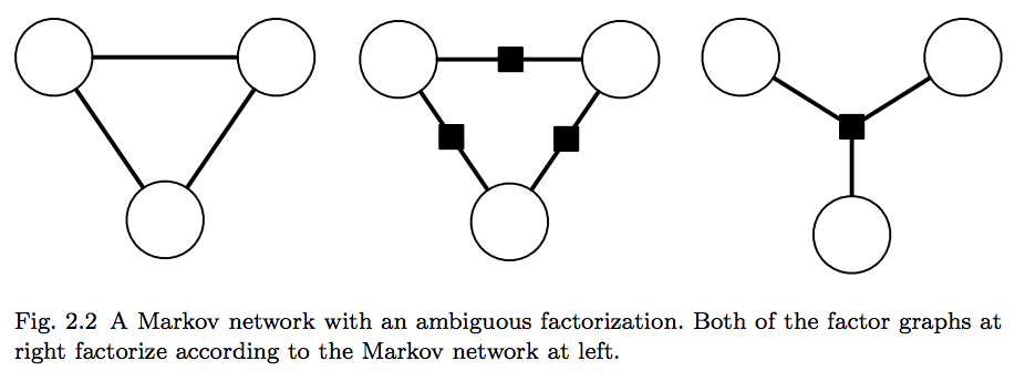
Any distribution that factorizes as  for some
positive function
for some
positive function  is Markov with respect to this graph. However, we
might want to represent the graph using a more restricted parameterization,
where
is Markov with respect to this graph. However, we
might want to represent the graph using a more restricted parameterization,
where  . This is a more strict
family of functions, and so one would expect it to be easier to estimate.
Unfortunately, as we can see in the figure, Markov networks doesn't really
distinguish between these cases. Lucky us, factor graphs do!
. This is a more strict
family of functions, and so one would expect it to be easier to estimate.
Unfortunately, as we can see in the figure, Markov networks doesn't really
distinguish between these cases. Lucky us, factor graphs do!
Directed Models
- Describes how the distribution factorizes into a local conditional probability distribution.
Inference
Belief propagation
Notation
- is the variable we want to compute the marginal distribution for
 is the neighborhood of *factors of , and it's the index of the neighboring factor of
  the set of variables "upstream" of , i.e. set of variables
  for which the factor is between and ( separates and ), with being the index of a neighboring factor of
  the set of factors "upstream" of , i.e. set of factors for which is between those and ("separates" from this set of factors), including the factor itself
Message from
to
Stuff
- Direct generalization of exact algorithms for Linear CRFs (i.e. Viterbi algorithm for sequences and Forward-backward algorithm for joint distributions)
- Each neighboring factor of makes a multiplicative contribution to the marginal of , called a message
In the special case where our graph is a tree, the graph itself is a the one and only spanning tree, hence we partition the entire graph wrt. : the sets  form a partition of the variables in . In a bit simpler wording:
- You're looking at
- Choose some other variable (node in the graph)
- All variables between and are along a single path (i.e. only one possible way to traverse from to )
- Therefore, the sets
 form a partition of the variables in , where
  denotes the number of neighboring nodes of
 - Thus, we can split upt the summation required for the marginal into a product of independent subproblems
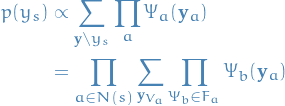
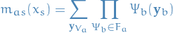
And denoting each of the factors in the above equation by  , i.e.,
which can be though of as a message from to .
And also, if instead take the product over neighboring factors, we can define the message from variables to factors as
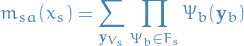
which would give us
Let's break this down:
 is product over all variables which are neighbors to the factor
  are all possible values the variables
  (i.e. "variables on one side of , including ") can take on
 is the product over all neigboring factors
  of the variable , excluding itself (which is our "focus" at the moment)
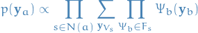
Observe that when talking about the "marginal for a factor ", we're looking at the marginal of a vector rather than a single value as in the marginal for a variable.
 denotes the vector of random variables with which are incoming to , NOT the distribution over the output of
Luckily, we can rewrite the messages recursively
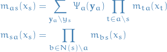
These recursion-relations define the belief propagation algorithm.
Belief progagation is the algorithm defined by the following recursion relations:
In the case where the graph is not a tree, we do not have the guarantee of convergence and refer to this algorithm as loopy belief propagation, as we can still find a fixed point.
As it turns out, Loopy BP can in fact be seen as a variational method, meaning that there actually exists an objective function over beliefs that is approximately minimized by the iterative BP procedure.
Appendix A: Vocabular
- random field
- a particular distribution among those defined by an unidirected graphical model
- biparite graph
- set of graph vertices decomposed into two disjoint sets s.t. no two graph vertices from the same set are adjacent / "directly connected".
- markov blanket
- simply a fancy word for the independent neighbors
- multivariate distribution
- distribution of multiple variables
Appendix B: Discriminative vs. Generative methods
- Discriminative model
- attempts to model
 , and thus indirectly model
  using Bayes'
 - Generative model
- attemps to model directly
First, it's very hard (impossible?) to tell beforehand whether a generative or discriminative model will perform better on a given dataset. Nonetheless, there are some benefits/negatives to both.
Benefits of discriminative:
- Agnostic about the form of

- Make independence assumptions among and how depend on
 , but
do not make conditional independence assumptions between the $$s
, but
do not make conditional independence assumptions between the $$s - Thus, these models are better at suited for including rich, overlapping (dependent) features.
- Better probability estimates than generative models; consider a vector of features
 which we transform to repeat the features, like so
  .
Then train, say a Naive Bayes', on this data. Even though no new data has been added
(just added multiple completely correlated features), the model will be more confident
in the probability estimates, i.e.
.
Then train, say a Naive Bayes', on this data. Even though no new data has been added
(just added multiple completely correlated features), the model will be more confident
in the probability estimates, i.e.  will be further away from
  than
than  .
Note that his in a way demonstrates the independence assumption between the features which
is beeing made a generative model.
.
Note that his in a way demonstrates the independence assumption between the features which
is beeing made a generative model.
Benefits of generative model:
- More natural for handling latent variables, partially-labeled data, and unlabeled data. Even in extreme case of unlabeled data, generative models can be applied, while discriminative methods is less natural.
- In some cases, generative model can perform better, intuitively because
might have a smoothening effect on the conditional.
- If application of the model requires both prediction of future inputs as well as outputs, generative models is a good choice since they model the joint distribution, and so we can potentially marginalize over whatever we don't want to predict to obtain a prediction for our target variable (being input or output).
It may not be clear why these approaches are different, as you could convert from one to the other, both ways, using Bayes' rule.
TODO Ongoing work
One interesting way to look at it is as follows:
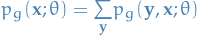
Suppose we have a generative model  which takes the form:
 3
3
And using the chain rule of probability we get
 4
4
where:
 is computed by inference
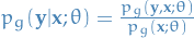 is computed by inference
And then suppose we another model, but this is discriminative model  :
:
Resources
Named Entity Recognition with a Maximum Entropy Approach A paper using MEMMs for word-tagging. I link this here since MEMMs are very similar to CRFs, but also because they provide a very nice set of features for use in word-tagging, which is something you might want to use CRFs for.
In fact, both CRFs and MEMMs are discriminative, unlike the generative HMMs, sequence models. Both CRFs and MEMMs are MaxEnt (maximum entropy) models, but a CRF is models the entire sequence while MEMMs makes decisions for each state independently of the other states.