Hidden Markov Models
Table of Contents
Model
Hidden Markov Model (HHM) is a probability model used to model latent
states (  ) based on observations which depends on the current
state of the system. That is; at some step
) based on observations which depends on the current
state of the system. That is; at some step  the system is in some
"internal" / unobservable / latent state . We then observe an
output
the system is in some
"internal" / unobservable / latent state . We then observe an
output  which depends on the current state, , the system is in.

Derivation
- Hidden states/rvs
 i.e. a discrete set of states
- Observed rvs

 is the set of all possible values that
  can take,
e.g. discrete,
can take,
e.g. discrete, 
Then,
 1
1
The reason why we use  here is that elements
of , can potentially be multi-dimensional, e.g.
here is that elements
of , can potentially be multi-dimensional, e.g.  ,
then
,
then  represents a vector of observed rvs, not just
a single observed rv.
represents a vector of observed rvs, not just
a single observed rv.
Parameters
- Transition probabilities/matrix:

- Emission probabilites:
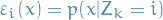 for
for 
 is then a prob. dist. on
- Initial dist:

The difference between  and
and  , e.g. lower- and uppercase notation
is that represents the distribution of the rv , while
is the actual rv, and so
, e.g. lower- and uppercase notation
is that represents the distribution of the rv , while
is the actual rv, and so  means the case where the rv
takes on the value
means the case where the rv
takes on the value  . The notation
  for some arbitrary
is then talking about a discrete distribution.
for some arbitrary
is then talking about a discrete distribution.
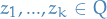
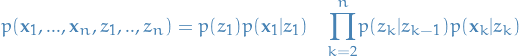
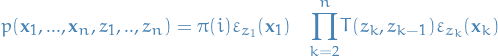
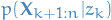
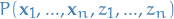
Using the substitutions from above, the join distribution is the following:
 2
2
The emission prob. dist for the different values of the hidden states can be basically any prob. dist.
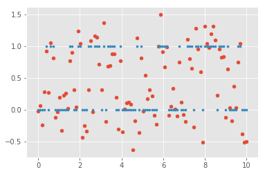
The plot below shows a problem where HMM might be a good application, where
we have the states  in
in blue and observations in red with
emission probability  .
.
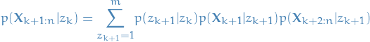
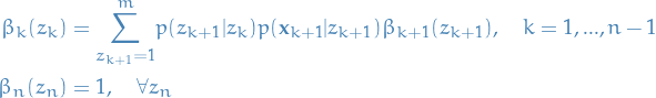
Forward-backward algorithm / alpha-beta recursion
Example of a dynamic programming algorithm. This provides us with a
way of efficiently estimating the probability of the system
being in some state at the  step given all
  observations we've seen,
  , i.e.
  .
.
This does not provide us with a way to calculate the probability of a sequence of states, given the observations we've seen. For that we have to have a look at the Viterbi algorithm.
Notation
 i.e. the sequence of observations made, not
the rv representing some
i.e. the sequence of observations made, not
the rv representing some  represents the sequence of observations from the
  observation to the
  observation
Algorithm
We make the assumptions that we know  ,
,  and
and  .
.
Our goal of the entire algorithm is to compute .
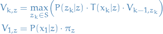
- Forward algorithm
- computes
 for all
- Backward algorithm
- computes
 for all
We can write our goal in the following way:
 3
3
Which means that if we can solve the forward and backward algorithms
described above, we can compute .
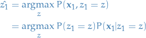
What we're actually saying here is:
- Given that we know the value of the rv. the sequence of
observations
 does not depend on the
observations prior to the observation.
does not depend on the
observations prior to the observation. - Observations prior to the observation, does not
depend on the observations in the future
Forward algorithm
Our goal is to compute .
We start out with the following:
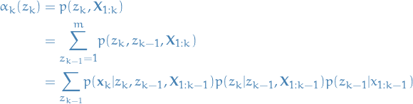 4
4
In words: probability of observing given that we have observed
the sequence  and we're in state marginalized / summed over
the possible previous states
and we're in state marginalized / summed over
the possible previous states  .
.
But since the observation at the step, , is independent of
given that we know . And so we have:
 5
5
And the state, , is independent of the previous observations
given that we know . And so further we have:
 6
6
Thus, we end up with:
 7
7
And if you go back to our assumptions you see that we have assumed
that we know the emission probabilities  and
the transition probabilities
and
the transition probabilities  . And thus we only have
one unknown in our equation.
. And thus we only have
one unknown in our equation.
Tracking this recursive relationship all the way back to the  ,
we end up with zero unknowns, since we also assumed to know the
initial probability .
,
we end up with zero unknowns, since we also assumed to know the
initial probability .
So just to conclude:
 8
8
provides us with the enough info to compute in a recursive
manner.
Time complexity
- For each step
 we have to sum over the
  possible
values for the previous state , and so this
is of time complexity
possible
values for the previous state , and so this
is of time complexity 
- But we have to do the step above for every possible value of ,
thus we have an additional
- Finally, we gotta do of these steps, and so we have the two
steps above with total time complexity
 being computed
times, leading us the time complexity of the Forward algorithm
to be
being computed
times, leading us the time complexity of the Forward algorithm
to be 
This is cool as it is linear in the number of steps, !
Backward algorithm
Our goal is to compute for all .
And again we try to deduce some recursive algorithm.
We start out with:
 9
9
Then if we simply define some auxilary variable  to
be
to
be
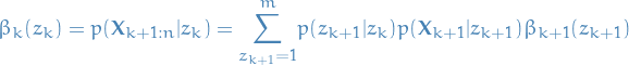 10
10
Aaaand we got ourselves a nice recursive relationship once again!
Again, by assumption, we know what 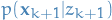 and
and  is.
is.
And the final step is as follows
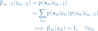 11
11
Thus, we conclude the Backward algorithm with the following:
 12
12
Time complexity
Again we have the same reasoning as for the forward algorithm time complexity
and end up with time complexity of .
Implementation
Throughout this implementation we will be validating against this wikipedia example.
First we gotta turn those data representations into structures which our implementation can work with:
wiki_emission_probs = np.array([[0.9, 0.1], [0.2, 0.8]])
wiki_initial_dist = np.array([[0.5, 0.5]])
wiki_observations = np.array([0, 0, 1, 0, 0])
wiki_transition_probs = np.array([[0.7, 0.3], [0.3, 0.7]])

S_wiki = np.arange(2)
T_wiki = wiki_transition_probs
X_wiki = wiki_observations
epsilon_wiki = lambda z, x: wiki_emission_probs[z][x]
pi_wiki = np.array([0.5, 0.5])
Forward
cnt = 0


def forward(pi, X, S, epsilon, T):
    n_obs = len(X)
    n_states = len(S)

    alpha = np.zeros((n_obs + 1, n_states))
    alpha[0] = pi

    for k_minus_one, x in enumerate(X):
        # readjust the index of alpha since
        # we're including pi too
        k = k_minus_one + 1

        alpha_k = alpha[k]

        for z_k in S:
            alpha_k[z_k] = sum(
                # p(z_k | z_{k-1}) * p(x_k | z_k) * alpha_{k-1}(z_{k-1})
                T[z, z_k] * epsilon(z_k, x) * alpha[k - 1][z]
                for z in S
            )

        # gotta normalize to get probab p(z_k, x_{1:k})
        alpha[k] = alpha_k / alpha_k.sum()

    return alpha

forward(pi_wiki, X_wiki, S_wiki, epsilon_wiki, T_wiki)
array([[ 0.5       ,  0.5       ],
       [ 0.81818182,  0.18181818],
       [ 0.88335704,  0.11664296],
       [ 0.19066794,  0.80933206],
       [ 0.730794  ,  0.269206  ],
       [ 0.86733889,  0.13266111]])
YAY!
Backward
cnt = 0


def backward(X, S, epsilon, T):
    n_obs = len(X)
    n_states = len(S)
    beta = np.zeros((n_obs + 1, n_states))  # 1 extra for initial state

    beta[0] = np.ones(*S.shape)
    beta[0] /= beta[0].sum()

    for k_plus_one in range(n_obs):  # n-1, ..., 1
        k = k_plus_one + 1               # iterating backwards yah know
        beta_k = beta[k]                       # just aliasing the pointers
        beta_k_plus_one = beta[k_plus_one]     # beta_{k+1}
        x_plus_one = X[k_plus_one]       # x_{k+1}

        for z_k in S:                    # for each val of z_k
            beta_k[z_k] = sum(
                # p(z_{k+1} | z_k) * p(X_{k+1} | z_{k+1}) * beta_{k+1}(z_{k+1})
                T[z_k, z] * epsilon(z, x_plus_one) * beta_k_plus_one[z]
                for z in S               # z_{k+1}
            )

            # validating the time complexity
            global cnt
            cnt += n_states

        # normalize the beta over the z's at each stage
        # since it represents p(x_{k+1:n} | z_k)
        beta_k = beta_k / beta_k.sum()

    # finally we gotta get the probabilities of the intial state
    x = X[0]
    for z_1 in S:
        beta[-1][z_1] = sum(T[z_1, z] * epsilon(z, x) * beta[-2][z] for z in S)

    # and normalize this too
    beta[-1] /= beta[-1].sum()

    # reversing the results so that we have 0..n
    return beta[::-1]

backward(X_wiki, S_wiki, epsilon_wiki, T_wiki)
array([[ 0.64693556,  0.35306444],
       [ 0.03305881,  0.02275383],
       [ 0.0453195 ,  0.0751255 ],
       [ 0.22965   ,  0.12185   ],
       [ 0.345     ,  0.205     ],
       [ 0.5       ,  0.5       ]])
Which is the wanted result! Great!
I find it interesting that the forward and backward algorithms
provide me with similar, but slightly different answers when we run
both of them independently on all of our observations.
BRAINFART! The forward algorithm aims to compute
the joint distribution  , while the
backward algorithm computes the conditional  , in the
case where we give the algorithms all the observations. They're not
computing the same thing, duh.
, in the
case where we give the algorithms all the observations. They're not
computing the same thing, duh.
And just to validate the time-complexity:
print "Want it to be about %d; it is in fact %d" % (len(X) * len(S_wiki), cnt)
Want it to be about 400; it is in fact 20
Forward-backward
Now for bringing it all together: forward-backward.
cnt = 0


def forward_backward(pi, X, S, epsilon, T):
    n_obs = len(X)
    n_states = len(S)

    posterior = np.zeros((n_obs + 1, n_states))

    forward_ = forward(pi, X, S, epsilon, T)
    backward_ = backward(X, S, epsilon, T)

    for k in range(n_obs + 1):
        posterior[k] = forward_[k] * backward_[k]
        posterior[k] /= posterior[k].sum()

    return posterior

forward_backward(pi_wiki, X_wiki, S_wiki, epsilon_wiki, T_wiki)
array([[ 0.64693556,  0.35306444],
       [ 0.86733889,  0.13266111],
       [ 0.82041905,  0.17958095],
       [ 0.30748358,  0.69251642],
       [ 0.82041905,  0.17958095],
       [ 0.86733889,  0.13266111]])
Eureka! We got the entire posterior distribution of the hidden states given the observations!
Discussion
Even though the plot looks nice and all, it seems weird to me
that everyone seems to be talkin about issues with underflow
while I'm getting overflow issues when dealing with large n o.O
I wasn't normalizing at each step, but instead waited until I had all the values and then normalized. Which means that I would get insanely large values of alpha, and thus doom.
I'm not 100% but I think it would still be a probability distribution
in the end, if, you know, I could get to the end without overflow error…
Example
predicted = []
posterior = forward_backward(pi, X, S, epsilon, T)

for p in posterior:
    predicted.append(np.argmax(p))
plt.scatter(steps, X, s=25)
plt.scatter(steps, zs, s=10)
plt.scatter(steps, predicted[:-1], alpha=0.1, c="g")
plt.title("%d samples" % n)

Here you can see the actual states plotted in blue,
the normally distributed observations in red, and
the predictions of the hidden states as a vague green.
Yeah, I should probably mess with the sizes and colors
to make it more apparent..
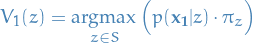
Viterbi algorithm
Allows us to compute the posterior probability
of a sequence of states,  , given some
sequence of observations,
, given some
sequence of observations,  .
.
Notation
- i.e. the sequence of observations made, not
the rv representing some
- represents the sequence of observations from the
observation to the observation
Algorithm
The main idea behind the Viterbi algorithm is to find the optimal / most probable sub-sequence at each step, and then find the optimal / most probable sub-sequence at the next step, using the previous steps optimal path.
The naive approach would be to simply obtain the probabilities
for all the different sequences of states,  given the sequence of observations
  .
The issue with this approach is quite clearly the number of
possible combinations, which would be
.
The issue with this approach is quite clearly the number of
possible combinations, which would be  , where
is the number of possible states.
, where
is the number of possible states.
A "dynamic programming" approach would be to attept to find a more feasible sub-problem and check if we can recursively solve these sub-problems, reducing computation by storing intermediate solutions as we go.

Wikipedia
So, let's start with the most likely intial path:
where
 , i.e. probability of first
state taking value
, i.e. probability of first
state taking value  , where
Our next step is then to define 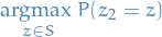 in terms of
The most likely state sequence  is given by the
recurrence relations:
is given by the
recurrence relations:
 13
13
where
 - probability of ???
 , i.e. probability of most
probable sequence of the first elements, given that the (entire?) path
ends in state .
, i.e. probability of most
probable sequence of the first elements, given that the (entire?) path
ends in state .
My interpretation
Viterbi algorithm is all about making locally optimal choices, storing this locally optimal sub-paths as you go, and reuse this computation when trying different choices of states.
You start out by the following:
Choose the initial state
s.t. you maximize the
probability of observing  , i.e.
 14
14
Now to the crucial part (and the part which makes this a dynamic programming algorithm!), we store both the probability of the sequence we've chosen so far and the states we've chosen. In this case, it's simply
 and
and 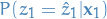 .
.
Choose the next state
 s.t. you maximize the
probability of observing
s.t. you maximize the
probability of observing  , conditioned
on already being in state , i.e.
, conditioned
on already being in state , i.e.
 15
15
And again, we store the current path and it's probability, i.e.
 and
and  .
Important: We store this somewhere else than
the first sub-path obtained, i.e.
.
Important: We store this somewhere else than
the first sub-path obtained, i.e.  and
and  .
.
- Perform this step until you reach the final step/observation,
i.e. times and you end up in
 .
.
Pretty complex, ehh? Simply choosing what seems the best at each step you take.
Now, let's think about the number of computations we got to do here.
- At each step we got to decide between possible states,
computing the probability
 for each one of them. This is required so that we know
which one to choose for our next state. That is; at each step
we do computations.
for each one of them. This is required so that we know
which one to choose for our next state. That is; at each step
we do computations. - We make the above choice until we reach the end, and so
we this is steps.
This leads us to a complexity of  , where
- is number of possible states
- is number of steps/observations
Unfortunately we're not done yet. We've performed
 operations, but what if the initial probability
of the state we chose first, , has "horrible"
probabilites as soon as you get past the first step?!
Maybe if we set equal to some other value, we
would get a much better probability in the end?
operations, but what if the initial probability
of the state we chose first, , has "horrible"
probabilites as soon as you get past the first step?!
Maybe if we set equal to some other value, we
would get a much better probability in the end?
Hence, smart as we are, we go "Okay, let's try again,
but this time we choose the second best initial state!".
And because we're running out of notation, we call this
 . Yeah I know, it's pretty bad, but you get the picture.
The
. Yeah I know, it's pretty bad, but you get the picture.
The  denotes that this is the 2nd try until we've
either realized that it's worse than our current ,
in which case we discard the new value, or we realize it's
in fact better, and so we simply replace it, i.e.
set
denotes that this is the 2nd try until we've
either realized that it's worse than our current ,
in which case we discard the new value, or we realize it's
in fact better, and so we simply replace it, i.e.
set  , also replacing the probability.
But how do we decide that the new suggested value is better? By walking through the path again, of course! But, this time we're going to try and be smart.
- If we at some step reach a node that we visited in our
first "walk", we don't have to keep going until the end,
but instead we terminate and do the following:
- Compare the probability of the sub-sequence
up until this step that we're currently looking at, with the
previous best estimate for this same sub-sequnce, i.e.
compare
 to
to  .
. If the new sub-path is more probable, then we replace our current best estimate for this sub-path, and recompute the joint conditional distribution for the rest of the path.
- Simply divide away our previous estimate, and multiply with
new and better sub-path probability:
 16
16
- Compare the probability of the sub-sequence
up until this step that we're currently looking at, with the
previous best estimate for this same sub-sequnce, i.e.
compare
For the sake of clarification, when we use the word
sub-path, we're talking about
a sequence of states  for some
  , i.e.
all sub-paths start at step
, i.e.
all sub-paths start at step  , ending at some . We're
not talking about sequences starting at any arbitrary .
, ending at some . We're
not talking about sequences starting at any arbitrary .
We repeat the process above for all possible initial states,
which gives us another factor of in the time-complexity.
This is due to having to perform the (possibly, see below)
 number of operations we talked about earlier for each
initial state, for which there are different ones.
number of operations we talked about earlier for each
initial state, for which there are different ones.
This means that, at worst, we will not reach any already
known / visited sequence, and so will do all the steps
for each possible initial state. For example, consider the case
of every state only being able to transition to itself.
In such cases we will have a
time complexity of  which is still substantially
better than
which is still substantially
better than  , the naive approach. But as I said, this
is worst case scenario! More often we will find
sub-sequences that we already have computed, and so we won't
have to do all the steps for every initial state!
, the naive approach. But as I said, this
is worst case scenario! More often we will find
sub-sequences that we already have computed, and so we won't
have to do all the steps for every initial state!
Thus, for the Viterbi algorithm we get a time complexity of
 (note Big-O, not Big-Theta)!
Implementation
First we need to set up the memoization part of the algorithm. Between each "attempt" we need to remember the following:
- At each step , the probability of most the likely sub-path.
We'll store as an array
best_sequence, with the the element pointing to an array of length , holding
the sequence/path of states for our best guess so far.
element pointing to an array of length , holding
the sequence/path of states for our best guess so far. - At each step , the state which was chosen by the most
likely sub-path. We'll store this in an array
best_sequence, with the element being the probability of the sequence/path
stored at best_sequence_probas[i].
n_obs = len(X_wiki)
n_states = len(S_wiki)

best_sequence = [None] * n_obs
best_sequence_probas = np.zeros(n_obs)

n_obs, n_states
| 5 | 2 |
First we choose the "best" initial state as our
starting point, and then start stepping through.
Best initial state corresponds to maximize the
 over .
Notice how we're not actually computing real probabilities as we're not normalizing. The reason for this is simply that it is not necessary to obtain the most likely sequence.
x_1 = X_wiki[0]

z_hat = S[0]
z_hat_proba = epsilon_wiki(S[0], x_1) * pi_wiki[S[0]]

initial_step_norm_factor = z_hat_proba

for z in S_wiki[1:]:
    z_proba = epsilon_wiki(z, x_1) * pi_wiki[z]
    initial_step_norm_factor += z_proba

    if z_proba > z_hat_proba:
        z_hat = z
        z_hat_proba = z_proba

best_sequence[0] = 1
best_sequence_probas[0] = epsilon_wiki(1, x_1) * pi_wiki[1] / initial_step_norm_factor

best_sequence[0], best_sequence_probas[0]
| 1 | 0.18181818181818182 |
for i, x in enumerate(X_wiki):
    if i == 0:
        continue

    prev_sequence = best_sequence[i - 1]
    z_hat_prev = best_sequence[i - 1]
    z_hat_prev_proba = best_sequence_probas[i - 1]

    # initialize
    z_hat = S_wiki[0]
    z_hat_proba = T_wiki[z_hat_prev, z_hat] * epsilon_wiki(z_hat, x)

    step_norm_factor = z_hat_proba

    for z in S_wiki[1:]:
        z_proba = T_wiki[z_hat_prev, z] * epsilon_wiki(z, x)
        step_norm_factor += z_proba

        if z_proba > z_hat_proba:
            z_hat = z
            z_hat_proba = z_proba

    best_sequence[i] = z_hat
    best_sequence_probas[i] = z_hat_proba * z_hat_prev_proba / step_norm_factor

best_sequence, best_sequence_probas
| (1 0 1 0 0) | array | ((0.18181818 0.11973392 0.09269723 0.06104452 0.0557363)) |
When I started doing this, I wanted to save the sub-path at each step.
Then I realized that this was in fact not necessary, but we instead could
simply store the state  at step and the probability of the previous
best estimate for the sub-path being in state at step .
When we're finished, we're left with a sequence
at step and the probability of the previous
best estimate for the sub-path being in state at step .
When we're finished, we're left with a sequence  which is the best estimate.
If you don't remember; what we did previously was storing the entire
sub-path up until the current step, i.e. at step we stored the sequence
 , which is bloody unecessary. This would allow us to
afterwards obtain the best estimate for any path though, so that would be nice.
But whenever we would hit a better estimate for a previously obtained path,
we would have to step through each
, which is bloody unecessary. This would allow us to
afterwards obtain the best estimate for any path though, so that would be nice.
But whenever we would hit a better estimate for a previously obtained path,
we would have to step through each  element for the stored sub-paths
and replace them.
element for the stored sub-paths
and replace them.
That was our first run, now we gotta give it a shot for the second best one. Since, as mentioned before, we've assumed a uniform prior, we simply pick the next state.
curr_seq = [0]
curr_seq_probas = [epsilon_wiki(curr_seq[0], x_1) * pi[curr_seq[0]] / initial_step_norm_factor]

for i, x in enumerate(X_wiki):
    if i == 0:
        continue

    z_prev = curr_seq[i - 1]
    z_prev_proba = curr_seq_probas[i - 1]

    # initialize the argmax process
    z_next = S_wiki[0]
    z_next_proba = T_wiki[z_prev, z_next] * epsilon_wiki(z_next, x)

    step_norm_factor = z_next_proba

    for z in S_wiki[1:]:
        z_proba = T_wiki[z_prev, z] * epsilon_wiki(z, x)
        step_norm_factor += z_proba

        if z_proba > z_next_proba:
            z_next = z
            z_next_proba = z_proba

    curr_seq_proba = curr_seq_probas[i - 1] * z_next_proba / step_norm_factor
    curr_seq.append(z_next)
    curr_seq_probas.append(curr_seq_proba)

    # check if the rest of the path has been
    # computed already
    z_hat = best_sequence[i]
    if z_hat == z_next:
        # we've computed this before, and the rest
        # of the path is the best estimate we have
        # as of right now
        best_seq_proba = best_sequence_probas[i]
        if best_seq_proba < curr_seq_proba:
            # the new path is better, so we gotta
            # replace the best estimate
            best_sequence[:i + 1] = curr_seq
            # and the preceding probabilities
            best_sequence_probas[:i + 1] = curr_seq_probas

            # then we have to recompute the probabilities
            # for the rest of the best estimate path
            for j in range(i + 1, n_obs):
                best_sequence_probas[j] = curr_seq_proba * \
                         best_sequence_probas[j] \
                         / best_seq_proba

            print "We found a better one! Current is %f, new is %f" \
                % (best_seq_proba, curr_seq_proba)

        # since we've already computed the sub-path after this step
        # given the state we are currently in, we terminate
        break

curr_seq, curr_seq_probas
| 0 | 0 |
| 0.8181818181818181 | 0.7470355731225296 |
best_sequence, best_sequence_probas
| (0 0 1 0 0) | array | ((0.81818182 0.74703557 0.57835012 0.38086471 0.34774604)) |
This looks very good to me!
def viterbi(pi, X, S, epsilon, T):
    n_obs = len(X)

    # initialize
    best_sequence = [None] * n_obs
    best_sequence_probas = np.zeros(n_obs)

    x_1 = X[0]
    initial_marginal = sum(epsilon(z, x_1) * pi[z] for z in S)

    sorted_S = sorted(S, key=lambda z: epsilon(z, x_1) * pi[z], reverse=True)

    for z_1 in sorted_S:
        curr_seq = [z_1]
        curr_seq_probas = [epsilon(z_1, x_1) * pi[z_1] / initial_marginal]

        for i, x in enumerate(X):
            if i == 0:
                continue

            z_prev = curr_seq[i - 1]
            z_prev_proba = curr_seq_probas[i - 1]

            # Max and argmax simultaenously
            # initialize the argmax process
            z_next = S[0]
            z_next_proba = T[z_prev, z_next] * epsilon(z_next, x)
            step_marginal = z_next_proba

            for z in S[1:]:
                z_proba = T[z_prev, z] * epsilon(z, x)

                step_marginal += z_proba

                if z_proba > z_next_proba:
                    z_next = z
                    z_next_proba = z_proba

            # Memoize our results
            curr_seq_proba = z_prev_proba * z_next_proba / step_marginal
            curr_seq.append(z_next)
            curr_seq_probas.append(curr_seq_proba)

            # check if the rest of the path has been computed already
            z_hat = best_sequence[i]
            if z_hat == z_next:
                # We've computed this before, and the rest
                # of the path is the best estimate we have.
                # Thus we check if this new path is better!
                best_seq_proba = best_sequence_probas[i]
                if best_seq_proba < curr_seq_proba:
                    # replace the best estimate sequence
                    best_sequence[:i + 1] = curr_seq
                    # and the corresponding probabilities
                    best_sequence_probas[:i + 1] = curr_seq_probas

                    # recompute the probabilities
                    # for the rest of the best estimate path
                    for j in range(i + 1, n_obs):
                        best_sequence_probas[j] = curr_seq_proba * \
                                 best_sequence_probas[j] \
                                 / best_seq_proba

                    print "We found a better one at step %d!" \
                                             "Current is %f, new is %f" \
                                             % (i, best_seq_proba, curr_seq_proba)

                # since we've already computed the sub-path after this step
                # given the state we are currently in, we terminate
                break

        # gone through all the observations for this state
        if i == n_obs - 1:
            best_seq_proba = best_sequence_probas[i]
            if best_seq_proba < curr_seq_proba:
                best_sequence = curr_seq
                best_sequence_probas = curr_seq_probas

    return best_sequence, best_sequence_probas
viterbi(pi_wiki, X_wiki, S_wiki, epsilon_wiki, T_wiki)
| 0 | 0 | 1 | 0 | 0 |
| 0.8181818181818181 | 0.7470355731225296 | 0.5783501211271196 | 0.3808647139129812 | 0.3477460431379394 |
Discussion
Using numpy.ndarray for curr_seq
I'm actually not sure whether or not this would speed up things.
The way Python list work provides us with a ammortized constant
time append method. This means that we can potentially save loads of
memory compared to having to preallocate memory for n_obs elements
using numpy.ndarray. Most of the time we won't be walking through
the entire sequence of observations, and so most of the memory allocated
won't even be used.
Nonetheless I haven't actually made any benchmarks, so it's all speculation. I just figured that it wasn't worth trying for the reason given here.
Python class implementation
Should this even be a class? I think it sort of makes sense, considering
it's kind of a model of a state machine. And so modelling it in a imperative
manner makes sense in my opinion.
Would it be a good idea to implement all of these as a
staticmethod, and then have the instance specific method
simply call the staticmethod? This would allow us to choose
whether or not we actually want to create a full instance of
a HiddenMarkovModel or not.
Naaah, we simply have functions which take those arguments
and then have the class HiddenMarkovModel call those methods.
Methods:
forwardbackwardforward-backwardviterbi
Properties:
posteriorepsilonandemission_probabilitiesTandtransition_probabilitiespiandinitial_probabilitiesSandstatesXandobservations
class HiddenMarkovModel:
    """
    A Hidden Markov Model (HMM) is fully defined by the
    state space, transition probabilities, emission probabilities,
    and initial probabilities of the states.

    This makes it easier to define a model, and then
    rerun it on different observations `X`.

    Parameters
    ----------
    pi: array-like floats, 1d
        Initial probability vector.
    S: array-like ints, 1d
        Defines the possible states the system can be in.
    epsilon: callable(z, x) -> float
        Takes current state :int:`z` and observation :float:`x`
        as argument, returning a :float: representing the
        probability of seeing observation :float:`x` given
        the system is in state :int:`z`.
    T: array-like floats, 2d
        Matrix / 2-dimensional array where the index `[i][j]`
        gives us the probability of transitioning from state
        `i` to state `j`.
    X: array-like (optional)
        Represents the observations. This can be a array-like
        structure of basically anything, as long as :callable:`epsilon`
        can handle the elements of `X`. So observations can be
        scalar values, vectors, or whatever.
    """
    def __init__(self, pi=None, S=None, epsilon=None, T=None, X=None):
        self.pi = pi
        self.S = S
        self.epsilon = epsilon
        self.T = T
        self.X = X

        # some aliases for easier use for others
        self.initial_probabilities = self.pi
        self.states = self.S
        self.emission_probabilities = self.epsilon
        self.transition_probabilities = self.T
        self.observations = self.X

        self.posterior = None
        self.optimal_path = None

    def forward(self, X=None):
        if X is None:
            X = self.X

        return forward(self.pi, X, self.S, self.epsilon, self.T)

    def backward(self, X=None):
        if X is None:
            X = self.X

        return backward(X, self.S, self.epsilon, self.T)

    def forward_backward(self, X=None):
        if X is None:
            X = self.X

        n_obs = len(X)
        n_states = len(S)

        posterior = np.zeros((n_obs + 1, n_states))

        forward_ = self.forward(X)
        backward_ = self.backward(X)

        for k in range(n_obs + 1):
            posterior[k] = forward_[k] * backward_[k]
            posterior[k] /= posterior[k].sum()

        # Should we actually set it, or leave that to the user?
        self.posterior = posterior

        return posterior

    def viterbi(self, X=None):
        if X is None:
            X = self.X

        self.optimal_path = viterbi(self.pi, X, self.S, self.epsilon, self.T)
        return self.optimal_path
hmm = HiddenMarkovModel(pi_wiki, S_wiki, epsilon_wiki, T_wiki)
hmm.viterbi(X_wiki)
hmm.forward_backward(X_wiki)

hmm.optimal_path
| 0 | 0 | 1 | 0 | 0 |
| 0.8181818181818181 | 0.7470355731225296 | 0.5783501211271196 | 0.3808647139129812 | 0.3477460431379394 |