Variational Inference
Table of Contents
Overview
In variational inference, the posterior distribution over a set of unobserved
variables  given some data
  is approximated by a variational distribution,
  :
:

The distribution  is restricted to belong to a family of
distributions of simpler form than
is restricted to belong to a family of
distributions of simpler form than  ,
selected with the intention of making similar to the true
posterior, .
,
selected with the intention of making similar to the true
posterior, .
We're basically making live simpler for ourselves by casting the approximate conditional inference as an optimization problem.
The evidence lower bound (ELBO)
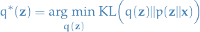
- Specify a family of densities over the latent variables
- Each
 is a candidate to the exact conditional distribution
 - Goal is then to find the best candidate, i.e. the one closest in KL divergence to the exact conditionanl distribution
 1
1
 is the best approx. to the conditional distribution, within that family
However, the equation above requires us to compute the log evidence
 which may be intractable, OR DOES IT?!
![\begin{equation*}
\begin{split}
\text{KL} \Big( q(\mathbf{z}) || p(\mathbf{z} | \mathbf{x}) \Big) &= \mathbb{E}_q[\log q(\mathbf{z})] - \mathbb{E}_q[\log p(\mathbf{z}|\mathbf{x})] \\
&= \mathbb{E}_q[\log q(\mathbf{z})] - \mathbb{E}_q[\log p(\mathbf{z}, \mathbf{x})] + \log p(\mathbf{x})
\end{split}
\end{equation*}](../../assets/latex/variational_inference_af40a8c3a2fff44965e91f388225a21d9d6423ec.png) 2
2
- Buuut, since we want to minimize wrt. , we can simply minizime the above, without
having to worry about !
- By dropping constant term (wrt.
 ) and moving the sign outside, we get
![\begin{equation*}
\text{ELBO}(q) = \mathbb{E}_q[\log p(\mathbf{z}, \mathbf{x})] - \mathbb{E}_q[\log q(\mathbf{z})]
\end{equation*}](../../assets/latex/variational_inference_9548be33807ca5988b0053f2bdff3f613d9f14eb.png) 3
3
- Thus, maximizing the
 is equivalent to minimizing the
  divergence
Why use the above representation of the ELBO as our objective function?
Because  can be rewritten as
  ,
thus we simply need to come up with:
,
thus we simply need to come up with:
- Model for the likelihood given some latent variables

- Some posterior probability for the latent variables
- We can rewrite the to give us a some intuition about the optimal variational density
![\begin{equation*}
\begin{split}
\text{ELBO}(q) &= \mathbb{E}_q[\log p(\mathbf{z})] + \mathbb{E}_q[\log p(\mathbf{x} | \mathbf{z})] - \mathbb{E}_q[\log q(\mathbf{z})] \\
&= \mathbb{E}_q[\log p(\mathbf{x} | \mathbf{z})] - \text{KL} \Big( q(\mathbf{z}) || p(\mathbf{z}) \Big)
\end{split}
\end{equation*}](../../assets/latex/variational_inference_15ccc87bf8a041ed5258c23354b244a51a12ddc0.png) 4
4
- Basically says, "the evidence lower bound of is the maximization of the likelihood and minimization of
the divergence from the prior distribution, combined"
![$\mathbb{E}_q[\log p(\mathbf{x} | \mathbf{z})]$](../../assets/latex/variational_inference_ee7133607f6a5d82af4a07e8df35b7aa7625cc0a.png) encourages densities that increases the likelihood
of the data
encourages densities that increases the likelihood
of the data encourages densities close to the prior
- Another property (and the reason for the name), is that it puts a lower bound on the (log) evidence,

 5
5
- Which means that if we increase the
 =>
=>  must decrease
Examples of families
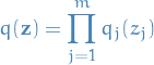
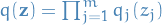
Mean-field variational family
- Assumes the latent variables to be mutually independent, i.e.
 6
6
- Does not model the observed data,
 does not appear in the equation
=> it's the which connects the fitted variational density to the data
does not appear in the equation
=> it's the which connects the fitted variational density to the data
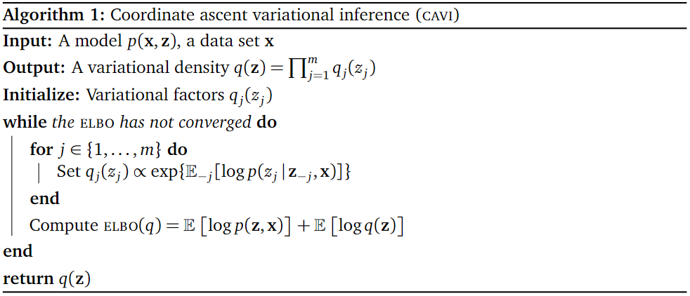
Optimization
Coordinate ascent mean-field variational inference (CAVI)
Notation
- is the data
- is the latent variables of our model for

 is the variational density
 is a variational factor
 , i.e. the
expectation over all factors of keeping the
, i.e. the
expectation over all factors of keeping the  factor constant
Overview
Based on coordinate ascent, thus no gradient information required.
Iteratively optimizes each factor of the mean-field variational density,
while holding others fixed. Thus, climbing the ELBO to a local optimum.
Algorithm
- Input: Model
 , data set
 - Output: Variational density
Then the actual algorithm goes as follows:
Psuedo implementation in Python
Which I believe could look something like this when written in Python:
import sys
import numpy as np


class UpdateableModel:
    def __init__(self):
        self.latent_var = np.random.rand(0, 1)

    def __call__(self, z):
        # compute q(z) or equivalently q(z_j | z_{l != j})
        # since mean-field approx. allows us to assume independence
        pass

    @staticmethod
    def proba_product(qs, z):
        # compute q_1(z_1) * q_2(z_2) * ... * q_m(z_m)
        res = 1
        for j in range(len(qs)):
            q_j = qs[j]
            z_j = z[j]
            res *= q_j(z_j)
        return res


def compute_elbo(q, p_joint, z, x, all_possible_vals=None):
    m = len(z)
    joint_expect = 0
    latent_expect = 0

    for j in range(m):
        q_j = q[j]
        z_j = z[j]

        joint_expect += q_j(z_j) * np.log(p_joint(z=z, x=x))
        latent_expect += q_j(z_j) * np.log(q_j(z_j))

    return joint_expect + latent_expect


def cavi(model, z, x, epsilon=5):
    """
    Parameters
    ----------
    model : callable
        Computes our model probability $p(z, x)$ or $p(z_j | z_{l != j}, x)$
    z : array-like
        Initialized values for latent variables, e.g. for a GMM we would have
        mu = z[0], sigma = z[1].
    x : array-like
        Represents the data.
    """
    m = len(z)
    q = [UpdateableModel() for j in range(m)]

    elbo = sys.maxint

    while elbo > epsilon:
        for j in range(m):
            # expectation for all latent variables
            expect_log = 0
            for j2 in range(m):
                if j2 == j:
                    continue
                expect_log += q[j2](z[j2]) * np.log(model(fixed=j, z=z, x=x))
            q[j].latent_var = np.exp(expect_log)

        elbo = compute_elbo(q, model, z=z, x=x)

    return q
Mean-field approx. → assume latent variables are independent of each other
→ can simply be represented as a vector with the entry being a
independent model correspondig to
Derivation of update
We simply rewrite the ELBO as a function of  , since the independence between
the variational factors implies that we can maximize the
, since the independence between
the variational factors implies that we can maximize the ELBO wrt. to each
of those separately.
![\begin{equation*}
\text{ELBO}(q_j) = \mathbb{E}_j \Big[ \mathbb{E}_{-j} \log p(z_j, \mathbf{z}_{-j}, \mathbf{x}) \Big] - \mathbb{E}_j [q_j ( z_j)] + \text{constant}
\end{equation*}](../../assets/latex/variational_inference_8e1ec13f115a71d40274e9c6c5476ffbd999ab1c.png) 7
7
Were we have written the expectation ![$\mathbb{E} [\log p(\mathbf{z}, \mathbf{x})]$](../../assets/latex/variational_inference_41e7bd9c8e6e93f3287e7f57d829ed50b0ab66da.png) wrt. using iterated expectation.
wrt. using iterated expectation.
Gradient
ELBO
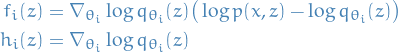
Used in BBVI (REINFORCE)
- Can obtain unbiased gradient estimator by sampling from the variational distribution
 without having to compute ELBO analytically
 - Only requires computation of score function of variational posterior:

Given by
![\begin{equation*}
\nabla_{\theta} \mathcal{L} = \mathbb{E}_{q_{\theta}} \big[ \nabla_{\theta} \log q_{\theta}(z) \big( \log p(x, z) - \log q_{\theta}(z) \big) \big]
\end{equation*}](../../assets/latex/variational_inference_009c454b5e3078d200341e71a06dec06b402db67.png)
- Unbiased estimator obtained by sampling from
- Unbiased estimator obtained by sampling from
Reparametrization trick
- needs to be reparametrizable
E.g.
 and
and

where
 and
and  are parametrized means and std. dev
Then we instead do the following:
![\begin{equation*}
\nabla_{\theta} \mathcal{L} = \mathbb{E}_{\varepsilon \sim r(\varepsilon)} \Big[ \nabla_{\theta} \Big( \log p\big(x, g(\varepsilon, \theta) \big) - \log q_{\theta} \big( g(\varepsilon, \theta) \big) \Big) \Big]
\end{equation*}](../../assets/latex/variational_inference_bbb5719bf5c34a83ceb3a2cec07885a0124d7843.png)
where
 is some determinstic function and
  is the "noise" distribution
- Observe that this then also takes advantage of the structure of the joint distribution
- But also requires the join-distribution to be differentiable wrt.

- But also requires the join-distribution to be differentiable wrt.
- Often the entropy of can be computed analytically which reduces the variance of the gradient estimate since we only have to estimate the expectation of the first term
Recall that
![\begin{equation*}
H(q_{\theta}) = \mathbb{E}_{z \sim q_{\theta}} \big[ \log q_{\theta}(z) \big] = \mathbb{E}_{\varepsilon \sim r(\varepsilon)} \big[ \log q_{\theta} \big( \underbrace{g(\varepsilon, \theta)}_{=: z} \big) \big]
\end{equation*}](../../assets/latex/variational_inference_1475b6740040b836801452d8ddc068e1e8d1202e.png)
- E.g. in ADVI where we are using Gaussian Mean-Field approx. which means that the entropy terms reduces to
 where
where 
- Assumptions
 must be differentiable
 must be differentiable
- Notes
 Usually lower variance than REINFORCE, and can potentially be reduced further if analytical entropy is available
- Not atually guaranteed zhang17_advan_variat_infer
 Being reparametrizable (and this reparametrization being differentiable) limits the family of variational posteriors
- Work towards using Gumbel-Max trick and replacing argmax operation with softmax operator for categorical distributions jang16_categ_repar_with_gumbel_softm
Differentiable lower-bounds of ELBO
- Aims to instead optimize lower-bounds of ELBO using more flexible variational posteriors
- E.g. SIVI yin18_semi_implic_variat_infer
Methods
- Automatic Differentiation Variational Inference (ADVI)
Objective:
![\begin{equation*}
\mathcal{L}(\mu, \omega) = \mathbb{E}_{\eta \sim \mathcal{N}(\mathbf{0}, \mathbf{I})} \bigg[ \log p \Big( \mathbf{X}, \big( T^{-1} \circ S_{\boldsymbol{\mu}, \boldsymbol{\omega}}^{-1} \big) (\eta) \Big) + \log \bigg( \left| \det \big( J(T^{-1} \circ S_{\boldsymbol{\mu}, \boldsymbol{\omega}}^{-1})\big|_{\eta} \big) \right| \bigg) \bigg] + \sum_{k=1}^{K} \omega_k
\end{equation*}](../../assets/latex/variational_inference_ab60623a8eb80cc53b2aa37c1de65fb942906530.png)
Gradient estimate:
![\begin{equation*}
\nabla_{\mu, \omega} \mathcal{L} \approx \frac{1}{M} \sum_{m=1}^{M} \nabla_{\mu, \omega} \bigg[ \log p \Big( \mathbf{X}, \big( T^{-1} \circ S_{\boldsymbol{\mu}, \boldsymbol{\omega}}^{-1} \big) (\eta_s) \Big) + \log \bigg( \left| \det \big( J(T^{-1} \circ S_{\boldsymbol{\mu}, \boldsymbol{\omega}}^{-1})\big|_{\eta_s} \big) \right| \bigg) + \sum_{k=1}^{K} \omega_k \bigg] \quad \text{where} \quad \eta_s \sim \mathcal{N}(0, I)
\end{equation*}](../../assets/latex/variational_inference_b9820e6ebdaac01515faf1657a5d07d910133508.png)
- Variational posterior:
- Gaussian Mean-field approx.
- Assumptions:
 is transformable in each component
 and
and  are independent
- Notes:
- If applicable, it just works
- Easy to implement
- Assumes independence
- Restrictive in choice of variational posterior
 (i.e. Gaussian mean-field)
- Black-box Variational Inference (BBVI)
Objective
![\begin{equation*}
\mathcal{L}(\theta) := \mathbb{E}_{z \sim q_{\theta}(z)} \big[ \log p(x, z) - \log q_{\theta}(z) \big]
\end{equation*}](../../assets/latex/variational_inference_f0a1e45c4f066003906e140a80cd2b22b90e604e.png)
Gradient estimate

Using variance reduction techniques (Rao-Blackwellization and control variate), for each
 ,
,

where
- Variational posterior
- Assumptions
- Notes
- Does not require differentiability of joint-density
- Gradient estimator usually has high variance, even with variance-reduction techniques
Automatic Differentiation Variational Inference (ADVI)
Example implementation
using ForwardDiff
using Flux.Tracker
using Flux.Optimise


"""
    ADVI(samplers_per_step = 10, max_iters = 5000)

Automatic Differentiation Variational Inference (ADVI) for a given model.
"""
struct ADVI{AD} <: VariationalInference{AD}
    samples_per_step # number of samples used to estimate the ELBO in each optimization step
    max_iters        # maximum number of gradient steps used in optimization
end

ADVI(args...) = ADVI{ADBackend()}(args...)
ADVI() = ADVI(10, 5000)

alg_str(::ADVI) = "ADVI"

vi(model::Model, alg::ADVI; optimizer = ADAGrad()) = begin
    # setup
    var_info = VarInfo()
    model(var_info, SampleFromUniform())
    num_params = size(var_info.vals, 1)

    dists = var_info.dists
    ranges = var_info.ranges

    q = MeanField(zeros(num_params), zeros(num_params), dists, ranges)

    # construct objective
    elbo = ELBO()

    Turing.DEBUG && @debug "Optimizing ADVI..."
    θ = optimize(elbo, alg, q, model; optimizer = optimizer)
    μ, ω = θ[1:length(q)], θ[length(q) + 1:end]

    # TODO: make mutable instead?
    MeanField(μ, ω, dists, ranges)
end

# TODO: implement optimize like this?
# (advi::ADVI)(elbo::EBLO, q::MeanField, model::Model) = begin
# end

function optimize(elbo::ELBO, alg::ADVI, q::MeanField, model::Model; optimizer = ADAGrad())
    θ = randn(2 * length(q))
    optimize!(elbo, alg, q, model, θ; optimizer = optimizer)

    return θ
end

function optimize!(elbo::ELBO, alg::ADVI{AD}, q::MeanField, model::Model, θ; optimizer = ADAGrad()) where AD
    alg_name = alg_str(alg)
    samples_per_step = alg.samples_per_step
    max_iters = alg.max_iters

    # number of previous gradients to use to compute `s` in adaGrad
    stepsize_num_prev = 10

    # setup
    # var_info = Turing.VarInfo()
    # model(var_info, Turing.SampleFromUniform())
    # num_params = size(var_info.vals, 1)
    num_params = length(q)

    # # buffer
    # θ = zeros(2 * num_params)

    # HACK: re-use previous gradient `acc` if equal in value
    # Can cause issues if two entries have idenitical values
    if θ ∉ keys(optimizer.acc)
        vs = [v for v ∈ keys(optimizer.acc)]
        idx = findfirst(w -> vcat(q.μ, q.ω) == w, vs)
        if idx != nothing
            @info "[$alg_name] Re-using previous optimizer accumulator"
            θ .= vs[idx]
        end
    else
        @info "[$alg_name] Already present in optimizer acc"
    end

    diff_result = DiffResults.GradientResult(θ)

    # TODO: in (Blei et al, 2015) TRUNCATED ADAGrad is suggested; this is not available in Flux.Optimise
    # Maybe consider contributed a truncated ADAGrad to Flux.Optimise

    i = 0
    prog = PROGRESS[] ? ProgressMeter.Progress(max_iters, 1, "[$alg_name] Optimizing...", 0) : 0

    time_elapsed = @elapsed while (i < max_iters) # & converged # <= add criterion? A running mean maybe?
        # TODO: separate into a `grad(...)` call; need to manually provide `diff_result` buffers
        # ForwardDiff.gradient!(diff_result, f, x)
        grad!(elbo, alg,q, model, θ, diff_result, samples_per_step)

        # apply update rule
        Δ = DiffResults.gradient(diff_result)
        Δ = Optimise.apply!(optimizer, θ, Δ)
        @. θ = θ - Δ

        Turing.DEBUG && @debug "Step $i" Δ DiffResults.value(diff_result) norm(DiffResults.gradient(diff_result))
        PROGRESS[] && (ProgressMeter.next!(prog))

        i += 1
    end

    @info time_elapsed

    return θ
end

function grad!(vo::ELBO, alg::ADVI{AD}, q::MeanField, model::Model, θ::AbstractVector{T}, out::DiffResults.MutableDiffResult, args...) where {T <: Real, AD <: ForwardDiffAD}
    # TODO: this probably slows down executation quite a bit; exists a better way of doing this?
    f(θ_) = - vo(alg, q, model, θ_, args...)

    chunk_size = getchunksize(alg)
    # Set chunk size and do ForwardMode.
    chunk = ForwardDiff.Chunk(min(length(θ), chunk_size))
    config = ForwardDiff.GradientConfig(f, θ, chunk)
    ForwardDiff.gradient!(out, f, θ, config)
end

# TODO: implement for `Tracker`
# function grad(vo::ELBO, alg::ADVI, q::MeanField, model::Model, f, autodiff::Val{:backward})
#     vo_tracked, vo_pullback = Tracker.forward()
# end
function grad!(vo::ELBO, alg::ADVI{AD}, q::MeanField, model::Model, θ::AbstractVector{T}, out::DiffResults.MutableDiffResult, args...) where {T <: Real, AD <: TrackerAD}
    θ_tracked = Tracker.param(θ)
    y = - vo(alg, q, model, θ_tracked, args...)
    Tracker.back!(y, 1.0)

    DiffResults.value!(out, Tracker.data(y))
    DiffResults.gradient!(out, Tracker.grad(θ_tracked))
end

function (elbo::ELBO)(alg::ADVI, q::MeanField, model::Model, θ::AbstractVector{T}, num_samples) where T <: Real
    # setup
    var_info = Turing.VarInfo()

    # initialize `VarInfo` object
    model(var_info, Turing.SampleFromUniform())

    num_params = length(q)
    μ, ω = θ[1:num_params], θ[num_params + 1: end]

    elbo_acc = 0.0

    # TODO: instead use `rand(q, num_samples)` and iterate through?

    for i = 1:num_samples
        # iterate through priors, sample and update
        for i = 1:size(q.dists, 1)
            prior = q.dists[i]
            r = q.ranges[i]

            # mean-field params for this set of model params
            μ_i = μ[r]
            ω_i = ω[r]

            # obtain samples from mean-field posterior approximation
            η = randn(length(μ_i))
            ζ = center_diag_gaussian_inv(η, μ_i, exp.(ω_i))

            # inverse-transform back to domain of original priro
            θ = invlink(prior, ζ)

            # update
            var_info.vals[r] = θ

            # add the log-det-jacobian of inverse transform;
            # `logabsdet` returns `(log(abs(det(M))), sign(det(M)))` so return first entry
            elbo_acc += logabsdet(jac_inv_transform(prior, ζ))[1] / num_samples
        end

        # compute log density
        model(var_info)
        elbo_acc += var_info.logp / num_samples
    end

    # add the term for the entropy of the variational posterior
    variational_posterior_entropy = sum(ω)
    elbo_acc += variational_posterior_entropy

    elbo_acc
end

function (elbo::ELBO)(alg::ADVI, q::MeanField, model::Model, num_samples)
    # extract the mean-field Gaussian params
    θ = vcat(q.μ, q.ω)

    elbo(alg, q, model, θ, num_samples)
end
Black-box Variational Inference (BBVI)
Stuff

Controlling the variance
- Variance of gradient estimator under MC estimation of ELBO) can be too large to be useful
Rao-Blackwellization
- Reduces variance of rv. by replacing it with its conditione expectation wrt. a subset of variables
- How
Simple example:
- Two rvs
 and
and 
- Function

- Goal: compute expectation
![$\mathbb{E} \big[ f(X, Y) \big]$](../../assets/latex/variational_inference_b7b59fdba8871e9cc8aece27a7babc97c30f6668.png)
Letting
![\begin{equation*}
\hat{f}(X) := \mathbb{E} \big[ f(X, Y) \mid X \big]
\end{equation*}](../../assets/latex/variational_inference_1f77521324638a46c1cb3b7dfb5558eac8f58159.png)
we note that
![\begin{equation*}
\mathbb{E} \big[ \hat{f}(X) \big] = \mathbb{E} \big[ f(X, Y) \big]
\end{equation*}](../../assets/latex/variational_inference_6f64c6d9c59e04911978f483c9f34baf8e2cd3ac.png)
Therefore: can use
 as MC approx. of , with variance
![\begin{equation*}
\Var \big( \hat{f}(X)\big) = \text{Var} \big( f(X, Y) \big) - \mathbb{E} \big[ \big( f(X, Y) - \hat{f}(X) \big)^2 \big]
\end{equation*}](../../assets/latex/variational_inference_b48cce185f6aba7f3c4c0d2c66df4f6b2dbf8813.png)
which means that
is a lower variance estimator than .
- Two rvs
- In this case
Consider mean-field approximation:
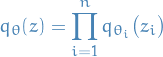
where
denotes the parameter(s) of variational posterior of  . Then the MC estimator for gradient wrt. is simply
But what the heck is
 ? Surely
  , right?
So you missed the bit where
 denotes the pdf of variables in the model that depend on the i-th variable, i.e. the Markov blanket of . Then
  is the joint probability that depends on those variables.
Important: model here refers to the variational distribution
! This means that in the case of a Mean-field approximation where the Markov blanket is an empty set, we simply sample  jointly.
Control variates
The idea is to replace the function
 being approximated by MC with another function
  which has the same expectation but lower variance, i.e. choose s.t.
![\begin{equation*}
\mathbb{E}[f(X)] = \mathbb{E}[\hat{f}(X)]
\end{equation*}](../../assets/latex/variational_inference_d36ac37141652e100a5eb83c8f43f0becd0b0149.png)
and

One particular example is, for some function
,
![\begin{equation*}
\hat{f}(z) := f(z) - a \big( h(z) - \mathbb{E} [h(z)] \big)
\end{equation*}](../../assets/latex/variational_inference_a1535c07db760ccc834d0bbc884b888d7917b1b7.png)
- We can then choose
 to minimize
Variance of
is then

- Therefore, good control variates have high covariance with
Taking derivative wrt.
and setting derivative equal to zero we get the optimal choice of , denoted  :
:
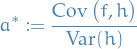
- We can then choose
Maybe you recognize this form from somewhere? OH YEAH YOU DO, it's the same expression we have for for the slope the ordinary least squares (OLS) estimator:
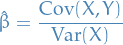
which we also know is the minimum variance estimator in that particular case.
We already know ![$\mathbb{E} [\hat{f}] = \mathbb{E}[f]$](../../assets/latex/variational_inference_d6556f637fb866c999e3f18bf2d756c08b39b070.png) , which in the linear case just means that the intercept are the same. If we rearrange:
, which in the linear case just means that the intercept are the same. If we rearrange:
![\begin{equation*}
\mathbb{E} [\hat{f}(Z)] + a \big( h(Z) - \mathbb{E}[h(Z)] \big) = \mathbb{E} [f(Z)]
\end{equation*}](../../assets/latex/variational_inference_1fcc73cefcb4b6a7bb255a7ff1bed9383a9bdfcf.png)
So it's like we're performing a linear regression in the expectation space, given some function  ?
?
Fun stuff we could do is to let be a parametrized function and then minimize the variance wrt. also, right future-Tor?
- This case
In this particular case, we can choose

This always has expectation zero, which simply follows from
![\begin{equation*}
\begin{split}
\mathbb{E} \big[ \partial_{\theta_i} \log q_{\theta}(z) \big] &= \int_{}^{} \big( \partial_{\theta_i} \log q_{\theta}(z) \big) q_{\theta}(z) \dd{z} \\
&= \int_{}^{} \frac{1}{q_{\theta}(z)} \pdv{q_{\theta}(z)}{\theta_i} q_{\theta}(z) \dd{z} \\
&= \int_{}^{} \pdv{q_{\theta}(z)}{\theta_i} \dd{z} \\
&= \pdv{}{\theta_i} \int_{}^{} q_{\theta}(z) \dd{z} \\
&= \pdv{}{\theta_i} 1 \\
&= 0
\end{split}
\end{equation*}](../../assets/latex/variational_inference_3e5a86cc109d803a29eda1c1ccb6ff6aaae8039d.png)
under sufficient restrictions allowing us to "move" the partial outside of the integral (e.g. smoothness wrt.
 is sufficient).
With the Rao-Blackwellized estimator obtained in previous section, we then have
The estimate of optimal choice of scaling
, is then
where
 and
and  denote the empirical estimators
 denotes the d-th component of
  , i.e. it can be multi-dimensional
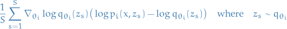
Therefore, we end up with the MC gradient estimator (with lower variance than the previous one):

Algorithm
![\begin{algorithm*}[H]
\KwData{data $x$, joint distribution $p$, mean-field variational family $q$}
\KwResult{posterior distribution $\hat{p}$}
\theta_{1:n} = random() \\
\While{not converged} {
\tcp{draw samples from variational distribution}
\For{$s = 1, \dots, S$} {
$z_s \sim q_{\theta}$
}
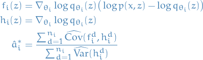
\For{$i = 1, \dots, n$} {
\For{$s = 1, \dots, S$} {
$f_i[s] := \nabla_{\theta_i} \log q_{i} (z_s) \big( \log p_i(x, z_s) - \log q_i(z_s) \big)$ \\
$h_i[s] := \nabla_{\theta_i} \log q_i(z_s)$
}
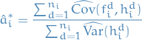
\tcp{compute scaling}
$\hat{a}_i^* := \frac{\sum_{d=1}^{n_i} \widehat{\Cov}(f_i^d, h_i^d)}{\sum_{d = 1}^{n_i} \widehat{\Var}(h_i^d)}$ \\
\tcp{lower-variance gradient estimator}
$\hat{\nabla}_{\theta_i} \mathcal{L} := \frac{1}{S} \sum_{s=1}^{S} f_i[s] - \hat{a}_i^* h_i[s]$
}
\tcp{update $\theta$}
$\dots$
}
\caption{Black-Box Variational Inference (BBVI)}
\end{algorithm*}](../../assets/latex/variational_inference_a2f3ad8eaf7074a42c5d8c937b4c782d68644301.png) 8
8
In the ranganath13_black_box_variat_infer as  where
where  is the t-th value of the Robbins-Monro sequence
Importance-weighted Autoencoder approach
Notation
Unnormalized importance weights
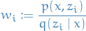
Normalized importance weights
Stuff
- burda15_impor_weigh_autoen
Proposes new objective
![\begin{equation*}
\mathcal{L}_k(x) = \mathbb{E}_{z_1, \dots, z_k \sim q_{\theta}(z)} \bigg[ \log \bigg( \frac{1}{k} \sum_{i=1}^{k} \frac{p(x, z)}{q_{\theta}(z_i \mid x)} \bigg) \bigg]
\end{equation*}](../../assets/latex/variational_inference_ef2e2389146716265135f150d51812c57882f1b0.png)
Lower bound on the marginal log-likelihood from the Jensen's Inequality and average importance weights is are unbiased estimator:
![\begin{equation*}
\mathcal{L}_k = \mathbb{E} \bigg[ \log \bigg( \frac{1}{k} \sum_{i=1}^{k} w_i \bigg) \bigg] \le \log \mathbb{E} \bigg[ \frac{1}{k} \sum_{i=1}^{k} w_i \bigg] = \log p(x)
\end{equation*}](../../assets/latex/variational_inference_91d0dfe363ba4530c79ab8f9d7f0a8ddc8e473d4.png)
where expectations are wrt.

Gradient
![\begin{equation*}
\begin{split}
\nabla_{\theta} \mathcal{L}_k(x) &= \mathbb{E}_{\varepsilon_1, \dots, \varepsilon_k} \bigg[ \sum_{i=1}^{k} \tilde{w}_i \nabla_{\theta} \log \Big( w\big(x, \underbrace{g(x, \varepsilon_i, \theta)}_{=: z_i}, \theta\big) \Big) \bigg]
\end{split}
\end{equation*}](../../assets/latex/variational_inference_8d78442d5b6accce92b19cc5a6d3d51411214691.png)
where we are using the reparamtrization trick with
being the reparametrization function
- This then has to be empirically approximated, e.g. sampling
 from
from  and computing the empirical estimate
- This then has to be empirically approximated, e.g. sampling
How to implement
- Could just implement an alternative objective function and take the gradient?
Appendix A: Definitions
- variational density
- our approximate probability distribution
- variational parameter
- a parameter required to compute our variational density, i.e. parameters which define the approx. distribution to the latent variables. So sort of like "latent-latent variables", or as I like to call them, doubly latent variables (•_•) / ( •_•)>⌐■-■ / (⌐■_■), Disclaimer: I've never called them that before in my life..
Bibliography
Bibliography
- [zhang17_advan_variat_infer] Zhang, Butepage, Kjellstrom, Hedvig & Mandt, Advances in Variational Inference, CoRR, (2017). link.
- [jang16_categ_repar_with_gumbel_softm] Jang, Gu & Poole, Categorical Reparameterization With Gumbel-Softmax, CoRR, (2016). link.
- [yin18_semi_implic_variat_infer] Yin & Zhou, Semi-Implicit Variational Inference, CoRR, (2018). link.
- [kucukelbir16_autom_differ_variat_infer] Kucukelbir, Tran, Ranganath, Rajesh, Gelman & Blei, Automatic Differentiation Variational Inference, CoRR, (2016). link.
- [kucukelbir15_autom_variat_infer_stan] Kucukelbir, Ranganath, Gelman, Andrew & Blei, Automatic Variational Inference in Stan, CoRR, (2015). link.
- [ranganath13_black_box_variat_infer] Ranganath, Gerrish, Blei & , Black Box Variational Inference, CoRR, (2013). link.
- [burda15_impor_weigh_autoen] Burda, Grosse, Salakhutdinov & Ruslan, Importance Weighted Autoencoders, CoRR, (2015). link.