Graphical models
Table of Contents
Notation
 denotes the parent nodes of the rv.
  in the BN
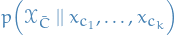
 denotes a clique
 denotes a set of variables in the clique
  are potential functions
Markov Random Fields
A Markov random field, also known as a Markov network or an undirected graphical model, has a set of nodes each of which corresponds to a variable or group of variables, as well as a set of links each of which connects a pair of nodes.
The links are undirected, i.e. do not carry arrows.
The Markov blanket of a node in a graphical model contains all the variables that "shield" the node from the rest of the network.
What this really means is that every set of nodes in a graphical model is conditionally independent of  when conditioned on the set
  , where denotes the Markov blanket of ; formally for distinct nodes and

In a Bayesian network, is simply the set of nodes consisting of:
- parents of
- children of
- parents of children of (these nodes are sometimes referred to has having a "explaining-away" effect)
Belief Network
A belief network is a distribution of the form
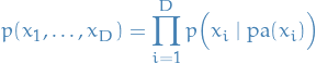
where  denotes the parental variables of variable
This can be written as a DAG, with the i-th node in the graph corresponding to the factor  .
.
Factorization properties
- Without loss of generality, only consider maximal cliques, since all other cliques are subsets
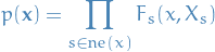
The joint distribution is written as a product of potential functions over the maximal cliques of the graph
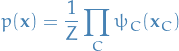
where the partition function is given by
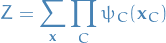
which ensures that the distribution  is correctly normalized.
To make a formal connection between the conditional independence and factorization for undirected graphs, we restrict attention to potential functions that are strictly positive, thus we can express them as:
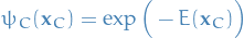
where  is called the energy function , and the exponential representation is called the Boltzmann distribution or Gibbs distribution.
A graph is said to be a D map (for dependency map) of a distribution if every conditional indepedence statement satisfied by the distribution is reflected in the graph.
Thus a completely disconnected graph (no links) wil l be a trivial D map for any distribution.
A graph is said to be a I map (for independence map) if every conditional independence statement implied by the graph is satisfied by a specific distribution.
Clearly a fully connected graph will be a trivial I map for any distribution.
If is the case that every conditional independence property of the distribution is reflected in the graph, and vice versa, then graph is said to be a perfect map.
Inference in Graphical Models
Notation
- denotes a variable (can be scalar, vector, matrices, etc.)
 denotes a subset of variables
  denotes the set of factor nodes that are neighbours of
 denotes the set of variables in the subtree connected to the variable node via a factor node
 denotes the set of variables in the subtree connected to the variable node
  via a factor node
 - f depends on
 , which we denote
  represents the product of all the factors in the group associated with factor
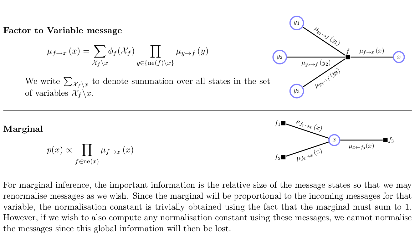
 Message from factor node
to variable node :
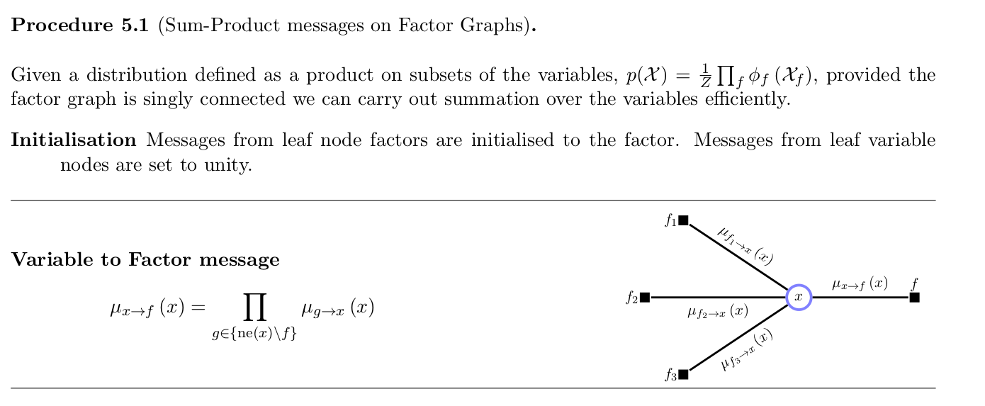
Message from variable node
to factor node :
where
denotes the set of factors in the subtree connected to the factor node via the variable node
Factor graphs
Can write joint distribution over a set of variables in the form of a product of factors
where
denotes a subset of the variables.
- Directed graphs represent special cases in which factors
 are local conditional distributions
 - Undirect graphs are a special case in which factors are potential functions over the maximal cliques (the normalizing coefficient
 can be viewed as a factor defined over the empty set of variables)
Converting distribution expressed in terms of undirected graph to factor graph
- Create variable nodes corresponding to the nodes in the original undirected graph
- Create additional factor nodes corresponding to the maximal cliques
- Factors are set equal to the clique potentials

There might be several factor graphs corresponding to the same undirected graph, i.e. this construction is not unique.
Sum-product algorithm
- Problem: evaluate local marginals over nodes or subsets of nodes
- Applicable to tree-structured graphs
- Exploit structure of the graph to achieve:
- efficient, exact inference algorithm for finding marginals
- in situations where several marginals are required to allow computations to be shared efficiently
- Summarized: barber2012
Belief propagation is a special case of sum-product algorithm, which performs exact inference on directed graphs without loops. (You have already written about this)
For actual implementation it's useful to use the logarithmic version of the messages. See barber2012.
Derivation
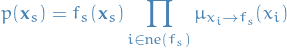
Marginal is obtained by summing the joint distribution over all variables except
so that
where
 denotes the set of variables in
  with the variable omitted.
Joint distribution of the set of variables
can be written as a product of the form
Rewriting the marginal above using the joint distribution notation:
![\begin{equation*}
\begin{split}
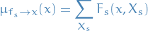
p(x) &= \prod_{s \in \text{ne}(x)} \Bigg[ \sum_{X_s} F_s(x, X_s) \Bigg] \\
&= \prod_{s \in \text{ne}(x)} \mu_{f_s \to x}(x)
\end{split}
\end{equation*}](../../assets/latex/graphical_models_b2ec044a3d4700dfce208b842605adccda639fa6.png)
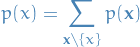
i.e. marginal is given by the product of all incoming messages arriving at node
.
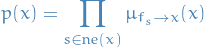
Each factor
can be descrbied by a factor (sub-)graph and so can itself be factorized:

where, for convenience, we have denoted the variable associated with factor
 , in addition to , by
  .
.
Message
to can be rewritten:
![\begin{equation*}
\begin{split}
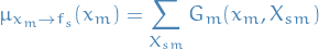
\mu_{f_s \to x} (x) & = \sum_{x_1} \dots \sum_{x_M} f_s(x, x_1, \dots, x_M) \prod_{m \in \text{ne}(f_s) \setminus x} \Bigg[ \sum_{X_{xm}} G_m(x_m, X_{sm}) \Bigg] \\
&= \sum_{x_1} \dots \sum_{x_M} f_s(x, x_1, \dots, x_M) \prod_{m \in \text{ne}(f_s) \setminus x} \mu_{x_m \to f_s}(x_m)
\end{split}
\end{equation*}](../../assets/latex/graphical_models_ed38558fbf9f5ab743f19ce60843b8599c35b751.png)
i.e. marginalizing over all the variables which
depend on, and the "messages" which are being sent from the variables to the factor . Thus, to evaluate message sent by factor to variable along the link connceting them:
- Take product of incoming messages along all other links coming into the factor node
- Multiply by the factor associated with that node
- Marginalize over all of the variables associated with the incoming messages
Message
to can be written:
![\begin{equation*}
\begin{split}
\mu_{x_m \to f_s}(x_m) &= \prod_{l \in \text{ne}(x_m) \setminus \left\{ f_s \right\}} \Bigg[ \sum_{X_{ml}} F_l(x_m, X_{ml}) \Bigg] \\
&= \prod_{l \in \text{ne}(x_m) \setminus \left\{ f_s \right\}} \mu_{f_l \to x_m}(x_m)
\end{split}
\end{equation*}](../../assets/latex/graphical_models_3226a6e5accea75ba4dc8de769bf7b441a1333a0.png)
i.e. to evaluate messages passed from variables to adjacent factors we simply take the product of incoming messages the incoming messages along all other links.
- Messages can be computed recursively
- Start: if leaf-node is:
variable: message it sends along its one and only link is given by
factor: message it sends is simply

- Start: if leaf-node is:
Finally, if we wish to find the marginal distributions
 associated with the sets of variables belonging to each factors:
Summarized
The sum-product algorithm can then be summarized as:
- Variable node is chosen as root of the factor graph
- Messages are initiaed at the leaves of the graph, if leaf is:
variable: message it sends along its one and only link is given by
factor: message it sends is simply
Message passing steps are applied recursively until messages have been propagated along every link:
![\begin{equation*}
\begin{split}
\mu_{f_s \to x} (x) & = \sum_{x_1} \dots \sum_{x_M} f_s(x, x_1, \dots, x_M) \prod_{m \in \text{ne}(f_s) \setminus x} \Bigg[ \sum_{X_{xm}} G_m(x_m, X_{sm}) \Bigg] \\
&= \sum_{x_1} \dots \sum_{x_M} f_s(x, x_1, \dots, x_M) \prod_{m \in \text{ne}(f_s) \setminus x} \mu_{x_m \to f_s}(x_m) \\
&= \sum_{X_s} F_s(x, X_s)
\end{split}
\end{equation*}](../../assets/latex/graphical_models_de527777dce5e0b8d981b548df9620f6c66785ca.png)
and
Once root node has received messages from all of its of its neighbors, the marginal can be evaluated by:
or, if one wants the marginal distribution
associated with the sets of variables belong to each of the factors:

- If we started from a:
- directed graph: already correctly normalized
undirected graph: started with unknown normalization constant
. From steps 1-4 we now have unnormalized marginal  , which we can marginalize over a single one of these (holding all other variables constant), which then gives us the normalization constant:
Could find marginals for every variable in the node in the graph by first passing messages from leaf to root, as in sum-product algorithm, and then when receiving all messages to the root, pass messages from the root back to the leaves.
Then we would have computed the messages along each of the links / edges in both directions, hence we could simply marginalize over these messages to obtain the wanted marginal.
Max-sum algorithm
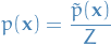
Problem: find most probable state or sequence:
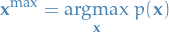
which will have the joint probability

- Summarized: barber2012
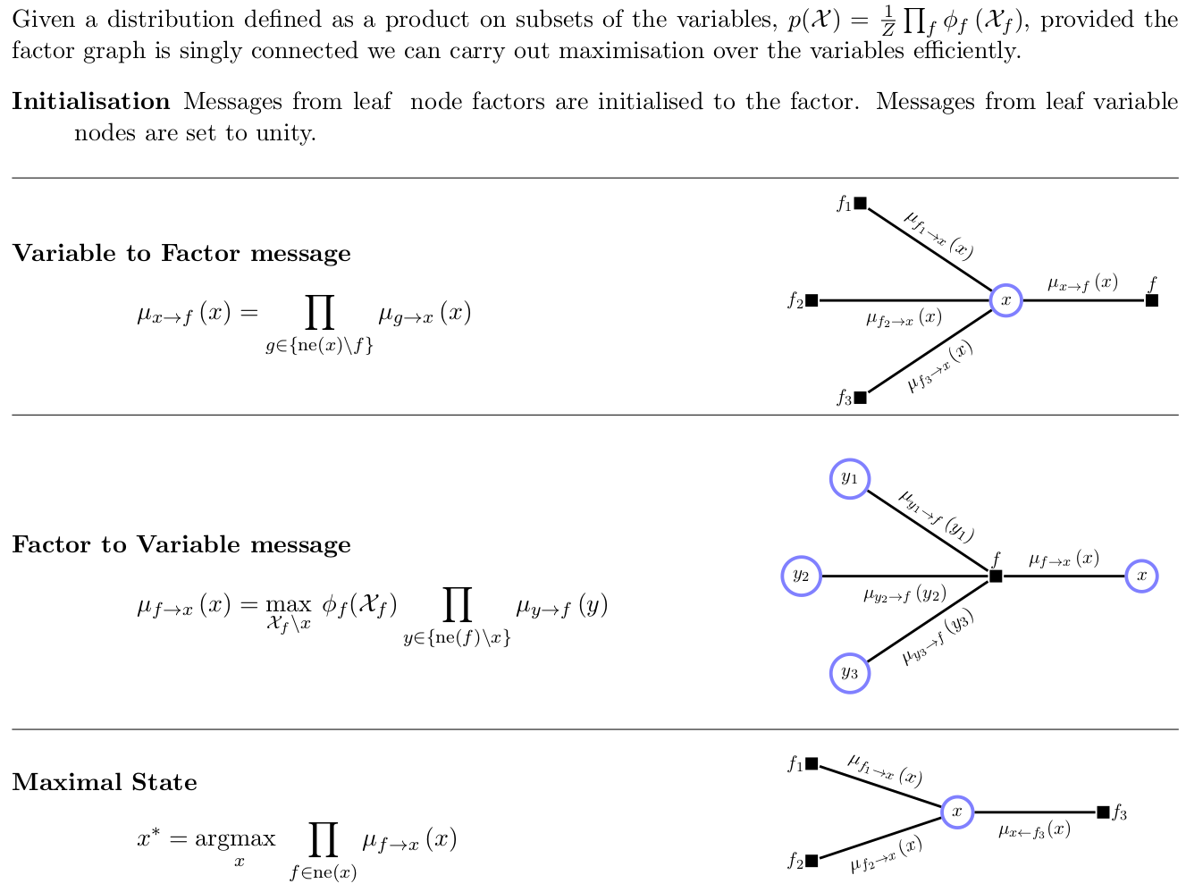
Figure 1: barber2012
Derivation
Will make use of

which holds if
 (always true for factors in graphical models!)
Work with
 instead (for numerical purposes), i.e.
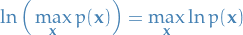
where the distributive property is preserved since

hence we replace products with sums.
Causality
In setting any variable into a particular state we need to surgically remove all parental links of that variable.
This is called the do operator, and constrants observational ("see") inference  with a casual ("make" or "do") inference
 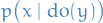 .
.
Formally, let all variables  be written in terms of the interventon variables
  and the non-intervention variables
  .
.
For a Belief Network 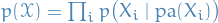 , inferring the effect of setting variables
  , in states
  , is equivalent to standard evidential inference in the post intervention distribution:

where any parental variable inclded in the intervention set is set to its intervention state. An alternative notation is
Intervention here refers to the "act of intervening", as in making some variable take on a particular state, i.e. we're interferring with the "total" state.
Bibliography
Bibliography
- [barber2012] Barber, Bayesian Reasoning and Machine Learning, Cambridge University Press (2012).