Optimization
Table of Contents
THE resource
Notation
Support of a vector
 is denoted by

A vector
 is referred to as s-sparse if
 denotes the number of zero-entries in
  denote A's singular values
Frobenius norm of

Nuclear norm of

Spectral norm of

- Random variables are denoted with upper-case letters

Definitions
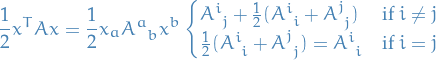
Algebraic Riccati equation
The (algebraic) Riccati equation is problem of finding an unknown matrix  in
in
Continuous case:

Discrete case:

where ,  ,
,  , and
, and  are known real coefficient matrices.
Lagrange multipliers
TODO Modern formulation via differentiable manifolds
Notation
 smooth manifold
 is a differentiable function we wish to maximize
 is a local chart
Stuff
By extension of Fermat's Theorem the local maxima are only points where the exterior derivative  .
.
In particular, the extrema are a subset of the critical points of the function  .
.
This is just a mapping from  to
to
Convex optimization
Visualization
Convexity
- Interpolation in codomain > interpolation in domain
using Plots, LaTeXStrings, Printf

f(x) = (x - 1) * (x - 2)
x₀, x₁ = 0., 6.


anim = @animate for t = 0:0.01:1
    z = (1 - t) * x₀ + t * x₁

    p = plot(-2:0.05:7, f, label="f(x)", legend=:topleft)
    # title!("Convexity: interpolation in codomain > interpolation in domain")
    vline!([z], label="", linestyle=:dash)
    scatter!([x₀, x₁], [f(x₀), f(x₁)], label="")
    plot!([x₀, x₁], f.([x₀, x₁]),
          label = L"(1 - t) f(x_0) + tf(x_1)",
          annotations = [(x₀ - 0.2, f(x₀), Plots.text(L"f(x_0)", :right, 10)), (x₁ + 0.2, f(x₁), Plots.text(L"f(x_1)", :left, 10))])
    scatter!([z], [f(z)],
             label="",
             annotations = [(z + 0.1, f(z), Plots.text(latexstring(@sprintf("f(%.2f x_0 + %.2f x_1)\\quad", (1 - t), t)), :left, 10))])
    scatter!([z], [(1 - t) * f(x₀) + t * f(x₁)],
             label = "",
             annotations = [(z - 0.1, (1 - t) * f(x₀) + t * f(x₁), Plots.text(latexstring(@sprintf("%.2f f(x_0) + %.2f f(x_1)\\quad", (1 - t), t)), :right, 10))])
end

gif(anim, "test.gif")
Definitions
A convex combination of a set of  vectors
  in an arbitrary real space is a vector
where:

A convex set is a subset of an affince space that is closed under convex combinations.
More specifically, in a Euclidean space, a convex region is a region where, for every pair of points within the region, every point on the straight line segment that joins the pair of points is also within the region, i.e. we say the set  is a convex set if and only if
![\begin{equation*}
\begin{split}
\forall \mathbf{x}, \mathbf{y} \in S, & \quad \lambda \in [0, 1] \\
(1 - \lambda) \mathbf{x} + \lambda \mathbf{y} & \in S
\end{split}
\end{equation*}](../../assets/latex/optimization_534f7ef9ae93527aece63d5a611b379bf327af65.png)
The boundary of a convex set is always a convex curve, i.e. curve in the Euclidean plane which lies completely on one side of it's tangents.
The intersection of all convex sets containing a given subset of Euclidean space is called the convex hull of , i.e. the smallest convex set containing the subset .
It's like a "convex closure" of .
A continuously differentiable function  is considered convex if

In more generality, a continuous function  is convex if for all
  ,
,

where the subscript of  emphasizes that this vector can depend on . Alternatively, if for all
  ,
,
![\begin{equation*}
f \Big( tx + (1 - t)y \Big) \le t f(x) + (1 - t) f(y), \quad \forall t \in [0, 1]
\end{equation*}](../../assets/latex/optimization_93e4cc9ce02b1d0ebc248c69c02500e7a5c3060c.png)
i.e. linear interpolation in input-space is "worse" than linear interpolation in output-space.
A continuously differentiable function is considered β-strongly convex
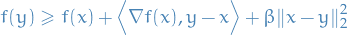
Similarily to a convex function, we don't require to be differentiable. In more generality, a contiuous function is β-strongly convex if for all and for all ![$t \in [0, 1]$](../../assets/latex/optimization_64ff94a722f22cff3ff97e2f423a713eb1e42c4e.png) we have nesterov2009primal
we have nesterov2009primal

Contrasting with the definition of a convex function, the only difference is the additional term  .
.
Quasi-convex and -concave
A quasiconvex function is a function  such that the preimage
  is a convex set.
To be precise, a function  defined on a convex set
  is quasiconvex if

for all  and
and ![$\lambda \in [0, 1]$](../../assets/latex/optimization_7cd670af2080b3c73aac2cd9f356000145119694.png) .
.
In words, is quasiconvex then it is always true that a point directly between two other points does not give a higher value of the function than both of the other points do.
A function is quasiconcave if we take the above definition and replace convex with concave and  with
with  .
.
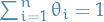
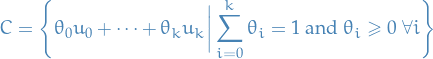
Simplex
A simplex is a generalization of the notion of a triangle or a tetrahedron to arbitrary dimensions.
Specifically, a k-simplex is a k-dimensional polytope which is the convex hull of its  vertices.
More formally, suppose the points  are affinely independent, which means
  are linearly independent. Then, the simplex determined by them is the set of points
Subgradient
Notation
 denotes the subgradient of
Stuff
We say  is a subgradient of
  at if
at if

where  replaces the gradient in the definition of a convex function.
Observe that the line 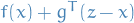 is a global lower bound of .
We say a function is subdifferentiable at if there exists at least one subgradient at .
The set of all subgradients at is called the subdifferential:  .
.
Some remarks:
- is convex and differentiable

 .
. - Any point , there can be 0, 1, or infinitely many subgradients.
 is not convex.
If  , then is a global minimizer of .
This is easily seen from definition of subgradient, since if  , then
 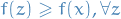 , i.e. global minimizer.
In general there might exist multiple global minimizers.
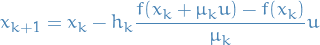
Subgradient Descent
- Suppose is convex, and we start optimizing at

- Repeat
Step in a negative subgradient direction:

where
 is the step-size and
  .
.
The following theorem tells us that the subgradient gets us closer to the minimizer.
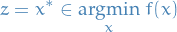
Suppose is convex.
- Let
 for
for - Let
 be any point for which
Then for small enough ,

i.e. it's a contraction mapping and it has a unique fixed point at
That is, the negative subgradient step gets us closer to minimizer.
Suppose is convex.
- Let for
- Let be any point for which
Then
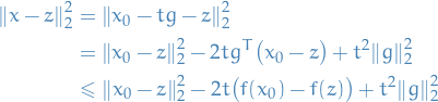
where we've used the definition a subgradient to get the inequality above.
Now consider 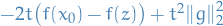 .
.
- It's a convex quadration (facing upwards)
Has zeros at
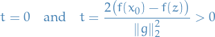
Therefore, due intermedite value theorem and convexity (facing upwards), we know the term above is negative if
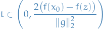
Hence,

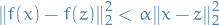
We then observe that if is Lipschitz, we have
with  , then the subgradient descent using a decreasing step-size is a contraction mapping with a fixed point at ! Hence,
If we're using a fixed step-size, we cannot guarantee the term considered in the proof of subgradient descent decreasing the objective function is negative (since at some point we get too close to , and so the fixed  we're using is not in the required interval).
That is why we use a decreasing step-size in the theorem above.
Using a fixed step-size, we still have the following bound
Cutting-plane method
- Used in linear integer programming
Consider an integer linear programming problem in standard form as

Gomory's cut
A Gomory's cut can be described geometrically as follows:
- Drop requirement for
 and solve resulting linear program
- Solution will be a vertex of the convex polytope consisting of all feasible points
- If this vertex is not an integer point
- Find a hyperplane with the vertex on one side and all feasible integer points on the other
- Add this as an additional linear constraint to exclude the vertex found
- Solve resulting linear program
- Goto Step 2.0
- Fin
One of my first thoughts regarding this was "But how the heck can you separate this vertex from all feasible points with a , since lin. prog. can't handle strict inequalities?!".
Solution: it says separating the vertex from all feasible INTEGER points, duh. This is definitively doable if the vertex is non-integer! Great:) Meza happy.
Non-convex optimization
Convex Relaxation
- Relax problem such that we end up with a convex problem
- E.g. relaxation of sparse linear regression, you end up with Lasso regression
- It's really
 regression, but as you can read on that link, it can be viewed as a approximation to the non-convex
  "norm",
  (it's not really a norm)
- It's really
- Can sometimes talk about the relaxation gap, which tells how different the optimal convex solution is from the non-convex
- Relaxation-approach can often be very hard to scale
TODO Convex Projections
- You're at Ch. 2.2 in jain17_non_convex_optim_machin_learn
Under uncertainty
Stochastic programming
Stochastic Linear Programming
A two-stage stochastic linear program is usually formulated as
![\begin{equation*}
\begin{split}
\min_x & c^T x + \mathbb{E}_{\omega} \big[ Q(x, \omega) \big], \quad x \in X \\
\text{subject to} & \quad Q(x, \omega) = \min f(\omega)^T y \\
& \quad D(\omega) y \ge h(\omega) + T (\omega) x, \quad y \in Y
\end{split}
\end{equation*}](../../assets/latex/optimization_658cdc1b5724dab781c2b4fcd872769f9fa9e170.png)
The first stage of the problem is the minimization above, which is performed prior to the realization of the uncertain parameter  .
.
The second stage is finding the variables  .
.
Linear quadratic programming
- Class of dynamic optimization problems
- Related to Kalman filter:
- Recursive formulations of linear-quadratic control problems and Kalman filtering both involve matrix Riccati equations
- Classical formulations of linear control and linear filtering problems make use of similar matrix decompositions
- "Linear" part refeers refers to the "motion" of the state
- "Quadratic" refers to the preferences
Stochastic optimization
TODO
Topics in Convex optimization
Lecture 1
Notation
- Black-box model: given input
 , a "oracle" returns
- Complexity of the algorithm is the number of queries made to the black-box oracle
Consider Lipschitz functions wrt. infinity-norm, i.e.
![\begin{equation*}
\mathcal{F}_L = \left\{ f : [0, 1]^n \to \mathbb{R} \mid \left| f(x) - f(y) \right| \le L \norm{x - y}_{\infty}, \quad \forall x, y \in [0, 1]^n \right\}
\end{equation*}](../../assets/latex/optimization_d56313aa4fae34d1eae54e5532cc9dfc3adf32d9.png)
Goal: find
![$\bar{x} \in [0, 1]^n$](../../assets/latex/optimization_589842b09c410412cf6613fbf28f1cac29510d32.png) s.t.
s.t.
Stuff
There is an algorithm with complexity  that can achieve the "goal" for all
  .
.
Grid search! Let  be the grid points, where
is then the number of grid points.
Query at the grid points . Find grid point  that achives the minimum of on
 ![$[0, 1]^n$](../../assets/latex/optimization_356f6940888678162faeb5ade5695e46b4094f4b.png) .
.
Let  be the closest grid point to

For any algo that acheives the "goal" for all , there exists an s.t. on , the algo will require at least  .
.
Gradient-based
Conjugate Gradient Descent (CGD)
Notation
 is such that

Resources
- [BROKEN LINK: No match for fuzzy expression: *GP%20&%20Kernel%20stuff]
Setup
Suppose we want to solve the system of linear equations

where

 is symmetric and positive-definitive
As it turns out, since is symmetric and positive-definite we can define an inner product wrt. :
We say two vectors  are conjugate if they are orthogonal wrt. inner product wrt. , i.e. if
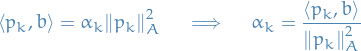
Method (direct)
Let

be a set of mutually orthogonal vectors (wrt. ), thus  forms a basis of
  .
.
We can therefore express  in this basis:
Let's consider left-multiplication  by
by  :
:
LHS can be written
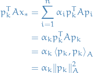
where we've let  denote the norm induced by the inner-product wrt. .
Therefore:
denote the norm induced by the inner-product wrt. .
Therefore:
Great! These solutions are exact, so why the heck did someone put the term "gradient" into the name?!
Because you might be satisfied with an approximation to the method if this would mean you don't have to find all of these "conjugate" / orthogonal (wrt. ) vectors! This motivatives writing it as a iterative method, which we can terminate when we get some  near the true solution.
Iterative
Observe that is actually the unique minimizer of the quadratic
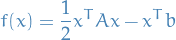
since

The fact that is a unique solution can then be seen by the fact that it's hessian

is symmetric positive-definite.
This implies uniqueness of solution only if we can show that
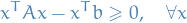
Since is positive-definite, we have

means that all <= NOT TRUE.
 .
.
Suppose  s.t.
s.t.  , which also implies
  by symmetry of . Then if
  and
and  for
for  , we have
If we let  , it is at least apparent that the diagonals of has to be non-negative.
What about when
, it is at least apparent that the diagonals of has to be non-negative.
What about when  ? Well, we then need

Since  are arbitrary, we require this to hold for all
  s.t.
s.t.  .
.
Great; that's all we need! Since for a symmetric real matrix we can do the eigenvalue decomposition of , i.e.

where  is a diagonal matrix with eigenvalues of as its entries, and
  is an orthonormal matrix. Thus

where we've let  . We can equivalently consider the case where
  and
and  for
for  . This then proves that the eigenvalues of a symmetric positive-definite matrix are all positive.
Gradient-free optimization
Random optimization
Idea
where
 is a random vector distributed, say, uniformly over the unit sphere
This converges under the assumption that  .
.
Mirrored descent
Suppose we want to minimize regret
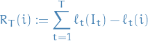
where
![$I_t \in [n]$](../../assets/latex/optimization_fe0eef89f1ab934ed8da0f02bbc9ac91a615ddcc.png) is a random variable indicating which index we chose as time
is a random variable indicating which index we chose as time ![$i \in [n]$](../../assets/latex/optimization_fdb5939c09c72a7b21153de66dbf7a6ebdceac18.png)
 indicating the loss of 0-1 loss of choosing the corresponding index
One approach is to solving this problem is to
- Define a discrete distribution over the indices
![$[n]$](../../assets/latex/optimization_af94be3ff4d5b20ec7ffd270dc20deb0bd4beb4c.png) , i.e.
, i.e.  .
. - Use gradient descent to find the optimal weights

TODO: watch first lecture to ensure that you understand the regret-bound for gradient descent
Doing the above naively, leads to the following bound
which unfortunately scales with dimensionality in  .
.
Mirrored descent takes advantage of the following idea:
- If we suppose there's one true optimal arm, say
 , then the resulting solution
  should be "sparse" in the sense that it should only have one non-zero entry, i.e.
  and
and  for
for  .
.
- Equivalently, will be a vertex in the simplex

- Equivalently,
- Naive gradient descent does not make use of this information → want to incorporate this somehow
There's an alternative approach: Franke-Wolfe is a convex-optimization algorithm which aims to point the gradient steps towards verticies.
This works very well for static problems, but in this formulation the function we're evaluating  is allowed to change wrt. , and apparently this is no good for Franke-Wolfe.