Graph Theory
Table of Contents
Notation
 denotes set of vertices in graph
  (
( is used when there is no scope for ambiguity)
 denotes set of edges in graph ( is used when there is no scope for ambiguity)
 and
and  denotes # of vertices and edges, respectively, unless stated otherwise
 denotes the incidence function which maps an edge to the set of vertices connected by this edge
 denotes the set of neigbours of a vertex
- A set , together with a set
 of two-element subsets of , defines a simple graph
  , where the ends of an edge
  are precisely the vertices
- incident matrix is
 matrix
  , where
  is # of times (0, 1, or 2) that vertex and egde
  are incident
 - adjacency matrix is
 matrix
  , where
  is # of edges joining
  and , with each loop counting as two edges
 - biparite adjaceny matrix of some biparite graph
![$G[X, Y]$](../../assets/latex/graph_theory_211101297abe6b757cad43363e18504619392036.png) is the
is the  matrix
  , where
  is # of edges joining
  and
and 
 denotes a sub-graph of some graph , i.e.
  (unless otherwise specified)
Definitions
Terminology
We say a graph is densily connected at vertex if  is "large".
If we have a cluster of such vertices, we might refer to this cluster as being assortative ; in contrast we refer to clusters of vertices which connect similarily to the rest of the graph (vertices "outside" of the cluster) without necessarily having higher inner density, as disassortative communities / clusters.
General
A tree is a undirected graph in which any two vertices are connected by exactly one path.
E.g. a acyclic connected graph is a tree.
Sometimes a tree also has the additional constraint that every node has at most a single parent, and polytrees refer to what we just defined.
A spanning tree  of an undirected graph is a subgraph that is a tree which includes all of the vertices of , with miniumum possible number of edges.
In general, a graph may have several spanning trees, but a graph that is not connected will not contain a spanning tree.
If all of the edges of are also edges of a spanning tree of , then is a tree and is identical to (i.e. a tree has a unique spanning tree and it's itself).
A cut is a partition of a the vertices of a graph into two disjoint subsets.
Any cut determines a cut-set, that is the set of edges which have one endpoint in each subset of the partition.
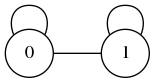
A simple graph is a graph where both multiple edges and self-loops are dissallowed.
Thus, in a simple graph with vertices, each vertex is at most of degree  .
.
Let  and
and  be two graphs.
Graph is a sub-graph of , written , if

If contains all of the edges  with
with  , then is an induced sub-graph of .
When  and there exists an isomorphism between the sub-graph
  and a graph , this mapping represents an appearance of in .
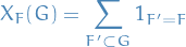
A graph is called recurrent or frequent in , when its frequency  is aboe a predefined threshold or cut-off value.
Intersection graph
An intersection graph is a graph that represents the pattern of intersections of a family of sets.
Formally, an intersection graph is an undirected graph formed from a family of sets

by creating one vertex  for each set
  , and connecting two vertices and
  by an edge whenever the corresponding two sets have a nonempty intersection, i.e.

Chordal graph
A chordal graph is one in which all cycles of 4 or more vertices have a chord, which is an edge that is not part of the cycle but connects two vertices of the cycle.
Sometimes these are referred to as triangulated graphs.
Network motifs
Network motifs are defined as recurrent and statistically significant sub-graphs or patterns in a graph.
There is an ensemble  of random graphs corresponding to the null-model associated to . We should choose
  random graphs uniformly from and calculate the frequency for a particular frequent sub-graph in .
If the frequency of in is higher than its arithmetic mean frequency in random graphs  , we acll this recurrent pattern significant and hence treat as a network motif for .
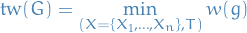
For a small graph , the network and a set of randomized networks  wher
wher  , the z-score of is defined as:
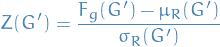
where  and
and  stand for mean and std. dev. frequency in set
  respectively.
The larger the  , the more significant is the sub-graph as a motif.
Clique
A clique is defined as a subset of nodes in a graph such that there exists a link between all pairs of nodes in the subset.
In other words, a clique is fully connected.
A maximal clique is a clique such that it is not possible to include any other nodes from the graph in the set without it ceasing to be a clique.
Theorems
Book: Graph Theory
1. Graphs
Notation
- denotes set of vertices in graph ( is used when there is no scope for ambiguity)
- denotes set of edges in graph ( is used when there is no scope for ambiguity)
- and denotes # of vertices and edges, respectively, unless stated otherwise
- denotes the incidence function which maps an edge to the set of vertices connected by this edge
- denotes the set of neigbours of a vertex
- A set , together with a set of two-element subsets of , defines a simple graph , where the ends of an edge are precisely the vertices
- incident matrix is matrix , where is # of times (0, 1, or 2) that vertex and egde are incident
- adjacency matrix is matrix , where is # of edges joining and , with each loop counting as two edges
- biparite adjaceny matrix of some biparite graph is the matrix , where is # of edges joining and
 denotes the degree of , i.e. # of edges incident with , each loop counting as two edges
 and
and  are the minimum and maximum degrees of the vertices of
  is the average degree of the vertices of
1.1 Graphs and Their Representations
A graph is an ordered pair  consisting of a set of vertices and a set , disjoint from , of edges, together with an incidence function
  that associates with each edge of an unordered pair of vertices of .
If is an edge and and are vertices such that  .
.
A biparite graph is a simple graph where the vertices can be partitioned into two subsets  and
and  such that every edge has one end in and one end in ; such a partition
  is called a bipartition of the graph, and and its parts.
A path is a simple graph whose vertices can be arranged in a linear sequence s.t. two vertices are adjacent if they are consecutive in the sequence, and are non-adjacent otherwise.
A cycle on three or more vertices in a simple graph whose vertices can be arranged in a cyclic sequence s.t. two vertices are adjacent if they are consecutive in the sequence, and are non-adjacent otherwise.
A graph is connected if and only if for every partition of its vertex set into two nonempty sets and , there is an edge with one end in and one end in ; otherwise the graph is disconnected.
Equivalently, if there is a u-v-path in (a path fro m to ) for every pair of vertices  .
.
A graph is k-regular if

A regular graph is one that is k-regular for some  .
.
Counting in two ways is a proof-technique where we consider a suitable matrix and compute the sum of its entries in two different ways:
- sum of its row sums
- sum of its column sums
Equating these two quantities results in an identity.
Exercises
- 1.1.5
- Question
For
 , characterize the k-regular graphs.
- Answer
Let
 , i.e.

which is simply a graph without any connections between the vertices.
For
 , we have

For any
we then the following possibilities:
- connected to itself, thus not connected to any other vertices, which in turn implies that we can consider two graphs;
 and
and 
- connected to another single vertex
 : a simple sequence of vertices, i.e. a path, since each vertex is connected only to one other
In total, a 1-regular graph can be separeted into graphs consisting of a single vertex with no edges (for all the vertices connected by loops) and a single graph which is a path.
For
 , we have

For any
we then have the following possibilities:
- both edges are loops: we can consider two graphs; and
- both edges are not loops: here we can have two cases
- is part of a cycle
 : can consider two separate graphs
  and
and  , since every
  is connected to two other vertices in
  for to form a cycle. is then simply a polygon
 - is not a part of a cycle: we have a simple graph
one edge is loop, one edge is non-loop:
can then only be connected to a single  which also has one loop and one non-loop, thus they form:
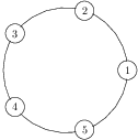
All in all, we can separate a 2-regular graph into graphs of the following classification:
- empty graphs
- k-cycles
- graphs of the form 1
- connected to itself, thus not connected to any other vertices, which in turn implies that we can consider two graphs;
- Question
Terminology
- loop
- edge with identical ends
- link
- edge with distinct ends
- parallel edges
- two or more links with the same pair of ends
- null graph
- graph with zero vertices
- trivial graph
- graph with one vertex
- complete graph
- simple graph in which any two vertices are adjacent
- empty graph
- simple graph in which no two vertices are adjacent, i.e.

- k-path
- path of length
- k-cycle
- cycle of length
- planar graph
- graph which can be drawn in a plane (2D) s.t. edges meet only at points corresponding to their common ends, i.e. no intersections when drawn in a 2D plane, where the drawing itself is called a planar embedding
- embedding
- "drawing" of a graph on some n-dimensional structure so that its edges intersect only at their ends
Book: Bayesian Reasoning and Machine Learning
Notation
 denotes the parent nodes of the rv. in the BN
7. Making Decisions
Notation
 denotes the expected utility of decision
  over the set of rvs.
7.3 Extending Bayesian Networks for Decisions
An Influence Diagram (ID) states which information is required in order to make each decision, and the order in which these decisions are to be made.
We call an information link fundamental if its removal would alter the partial ordering.
7.4 Solving Influence Diagrams
A decision potential on a clique  contains two potentials: a probability potential
  and a utility potential
  . The join potentials for the junction tree are defined as
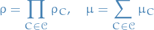
with the junction tree representing the term  .
.
But for IDs there are constraints on the triangulation since we need to preserve the partial ordering induced by the decisions, which gives rise to strong Junction Tree.
- Remove information edges
- Moralization: marry all parents of the remaining nodes
- Remove utility nodes: remove the utility nodes and their parental links
- Strong triangulation: form a triangulation based on an elimination order which obeys the partial ordering of the variables.
- Strong Junction Tree: From the strongly triangulated graph, form a junction tree and orient the edges towards the strong root (the clique that appears last in the eliminiation sequence).
Spectral Clustering
Notation
- denotes the i-th vertex
 when is adjacent to
  denotes the edge between and
 - Edges are non-negatively weighted with the weight matrix

- is the diagonal matrix of , also called the degree matrix, defined as:

 denotes the unnormalized graph Laplacian
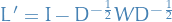 denotes the normalized graph Laplacian
Stuff
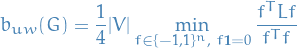
- Want to partition a graph in parts which are roughly the same size and are connected by as few edges as possible, or informally, "as disjoint as possible"
- NP-hard (even approximations are difficult)
- Good heuristic: write cost function as a quadratic form and relaxing the discrete optimization problem of finding the characteristic function of the cut to a real-valued optimization problem
- Leads to an eigenproblem
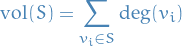
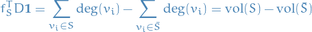
The volume of a subset of vertices  is the total degree of all vertices in the subset:
If is a set of vertices of , we define it's edge boundary  to be the set of edges connecting
  and its complement
  .
.
Similiarily, the volume of is defined as

The minimum cut of a graph refers to the partition  which minimizes
  , i.e. the smallest total weight "crossing" between the partitions and
  .
.
Problem with mincut is that no penalty is paid for unbalanced partitions and therefore nothing prevents the algorithm from making single vertices "clusters".
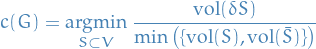
The Cheeger constant (minimum conductance) of a cut is defined
The normalized cut is defined as
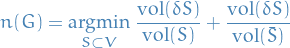
For  ,
,
from which we can see that Cheeger constant and normalized cut are closely related.
Both are NP-hard, thus need to be approximated.
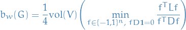
The weighted and unweighted , respectively, balanced cuts of a graph are given:
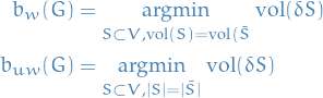
We'll assume balanced partitions exists (e.g. for unweighted version the number of vertices has to be even). For the general case one can easily modify the definition requiring the partition to be "almost balanced", and this will lead to the same relaxed optimization problems in the end.
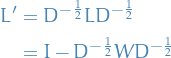
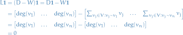
The unnormalized graph Laplacian is defined to be

and the normalized graph Laplacian
From  and
and  various graph invariants can be estimated in terms of eigenvalues of these matrices.
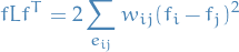
Given a vector  , we have the following identity:
thus is positive semi-definite, and since  is positive definite the same holds for .
Spectral clustering
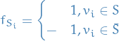
Given a subset , define the column vector  as follows:
Then it's immediate that
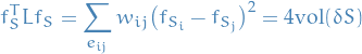
since  and
and  .
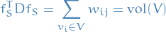
For all we have
.
For all we have
Consider the weighted balanced cut:
Hence,  if and only if the cut corresponding to is volume-balanced, i.e.

Therefore, we can reformulate the problem of computing weighted balanced cut as:

Moreover, as  has constant value
  for all
  , we can rewrite this as
I'll be honest and say I do not see where this  comes from.
In this form, the discrete optimization problem admits a simple relaxation by letting  instead of
  . Noticing that
a standard linear algebra argument shows that
I tried to figure out why "since  the minimizer is instead
  !" and what I can gather is that:
- means that the matrix is non-invertible
- Then only consider
 , i.e. subspace not spanned by eigenspace of
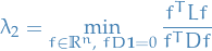
- Left with this stuff, which makes sense; the Rayleigh quotient is minimized by the first eigenvalue
where is the second smallest eigenvalue of the generalized eigenvector problem  . It is clear that the smallest eigenvalue of is
  (since
  as noted earlier) and the corresponding eigenvector is
  .
.
Further, we can show that for a connected graph,  . Thus, the vector
  for which the minimum above is attained is the eigenvector corresponding to .
This leads directly to the bipartitioning algortihm as relaxation of the weighted balanced cut:
- Compute the matrices and
Find the eigenvector corresponding to the second smallest eigenvalue of the following generalized eigenvalue problem:

Obtain the partition:

where  denotes the i-th entry of the corresponding eigenvector.
For unnormalized spectral clustering, a similar argument shows that
and by relaxation we obtain an identical algorithm, except taht the eigenproblem

is sovled instead.
Network Data Analysis
Notation
 denotes the linear space of all bounded symmetric measureable functions
 ![$[0, 1]^2 \to \mathbb{R}$](../../assets/latex/graph_theory_1a5f286271bacf248c029cc3cc6646edcfd01f21.png)
 is a kernel:
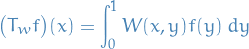
Considered as an operator
![$L_\infty[0, 1] \to L_1[0, 1]$](../../assets/latex/graph_theory_94410d9c0fef82e4ecafd3767ec5240ccc8a2f83.png)
![\begin{equation*}
\norm{T_W}_{\infty \to 1} = \sup_{f \in L_{\infty}[0, 1]: \norm{f}_\infty = 1} \norm{T_w f}_1
\end{equation*}](../../assets/latex/graph_theory_0c63778380a9f823acb9bd2a21ac86b346fb1563.png)
 is used to control sparsity
 is the
 is the expected number of occurences of subgraph
  in graph
 - "random graph" = Erdos-Renyi
Stuff
- Treating adjacency-matrix as a multi-dimensional Bernoulli rv. => allows possibility "construction" and "destruction" of connections
Real networks often follow:
Limiting behaviour

- Heterogenous:
 for some choices of
  or
or  and
and 
- No ordering
Hence, we consider the limiting behaviour
Graphons
A graphon is a symmetric measurable function ![$W: [0, 1]^2 \to [0, 1]$](../../assets/latex/graph_theory_ad939bc735caf4be8f9ef148566ab85cd762e055.png) .
.
Usually a graphon is understood as defining an exchangeable random graph model according to the following scheme:
- Each vertex
 of the graph is assigned an independent random value
 ![$u_j \sim U[0, 1]$](../../assets/latex/graph_theory_a3f407755cc9e2c71572c9f7fbfca7f6d4611c2e.png)
- Edge
 is independently included in the graph with probability
A random graph model is an exchangeable random graph model if and only if can be defined in terms of a (possibly random) graphon in this way.
It is an immediate consequence of this definition and the law of large numbers that, if  , exchangeable random graph models are dense almost surely.
Define a generative model of random graphs
- Fix a nonegative kernel and scale

- Generate iid Uniform(0, 1) variates

- Indep. connect vertices
 w.p.
w.p. 
Can we recover up to scale from an observed graph?
We therefore consider the cut distance, which can be defined naturally on the linera space of kernels.
Constructing an exchangeable model
Suppose we give  a univariate "prior" distribution

eqn scale the resulting mean matrix  by to control sparsity:
![\begin{equation*}
\mathbb{E}[A_{ij} \mid \pi ] = p_{ij} = \rho_n \cdot \pi_i \pi_j
\end{equation*}](../../assets/latex/graph_theory_fc2d992cdcecf69dfde666c3e0f220a41cdb6456.png)
Let  , then

where  is a "Kartauff effect" (?)
Stochastic block models
Assume each node is assigned categorical variable  :
:
![\begin{equation*}
\mathbb{E}[A_{ij} \mid z] = \theta_{ab} I(z_i = a) I(z_j = b)
\end{equation*}](../../assets/latex/graph_theory_05e13f0e5075965238b917f7216748a9bd1db15b.png)
The a-th fitted community then comprises  > 1 nodes:
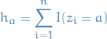
i.e. is the number of members in the community.
These "bandwiths" define a CDF  an its inverse
  .
.
Any community assignment function  has two components:
- A vector
 of community sizes (defines )
 - A permutation
 of
of  that re-orders the nodes prior to applying the quantile function
  .
.
Community to which assigns node  is determined by the composition
  :
:

Thus, each represents a re-ordering of the network nodes, followed by a partitioning of the unit interval.
Comparing features
- Inexact graph matching - maximum common subgraph, etc.
- Edit distance - convergence implies that motif prevalences converge also
- Motif prevelance
One way
Count prevalance of subgraph
in graph
- Compare to a null-model, typically moment matched (i.e. matching something like mean, variance, etc.)
- Compare subgraphs somehow
- Finite connected graph
 can be mapped out by a closed walk
  (i.e. sequence of vertices)
 - Walks in a network determine its classification as a topological space
- Euler characteristic:

- Number of closed k-walks in derives from its adjancey matrix:

- For large classes of networks, walks mapping out maximal trees and cycles dominate => allows comparison between "random graphs"
- Turns out that counting cycles allows one to determine whether or not we're just looking at a "random graph"; i.e. if the graph exhibits any interesting behavior or not
Tree decomposition
- Also called juntion trees, clique trees or join trees
Moralization of a graph is the process of turning a directed graph into an undirected graph by "marrying" of parent nodes.
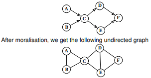
Figure 3: Source http://www.inf.ed.ac.uk/teaching/courses/pmr/slides/jta-2x2.pdf
Triangulation refers to the process of turning a graph into a chordal graph.
One of the reasons why this is so useful is when we turn triangulated graph into a clique tree for use in representing a factor graph.
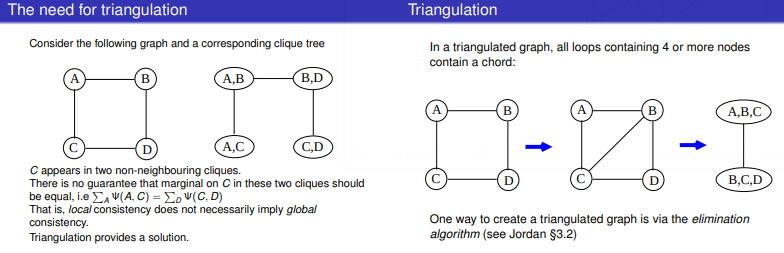
Figure 4: Source http://www.inf.ed.ac.uk/teaching/courses/pmr/slides/jta-2x2.pdf
A junction tree or tree decomposition represents the vertices of a given graph as subtrees of a tree, in such a way that the vertices in the given graph are adjacent only when the corresponding subtrees intersect.
Thus, forms a subgraph of the intersection graph of the subtrees. The full intersection graph is a chordal graph.
Given a graph , a junction tree is a pair 
 where
where  (in some literature referred to as "supernodes")
 is a tree whose nodes correspond to the subsets
  , i.e. a vertex
  is defined by
And this pair is required to satisfy the following:
 , i.e. each vertex is associated with at least one tree node in
 Vertices are adjacent in the graph
if and only if the corresponding subtrees have a node in common, i.e.

If
and  both contain a vertex , then all nodes
  of the tree in (unique) path between and contain as well, i.e.

where
 denotes the set of notes in the (unique) path between and
A junction tree is not unique, i.e. there exists multiple ways to perform a decomposition described above.
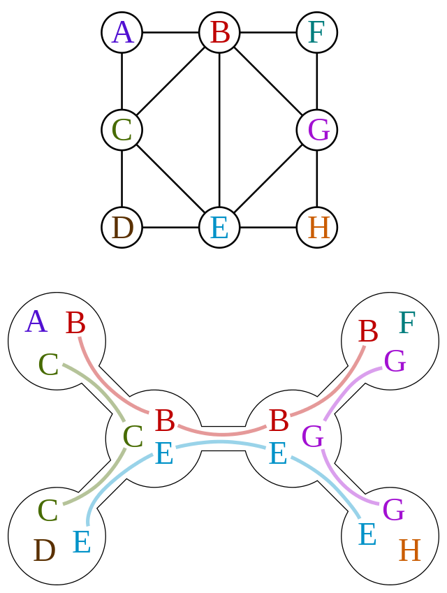
Figure 5: 
Often you'll see that it's suggested to transform a graph into a chordal graph before attempting to decompose it.
This is due to a theorem which states that the following two are equivalent:
- is triangulated
- Clique graph of has a junction tree
One method of exact marginalization in general graphs is called the junction tree algorithm, which is simply belief propagation on a modified graph guaranteed to be a tree.
The basic premise is to eliminate cycles by clustering them into single nodes.
Given a triangulated graph, weight the edges of the clique graph by their cardinality,  , of the intersection of the adjacent cliques
  and
and  . Then any maximum-weight spanning tree of the clique graph is a junction tree.
Thus, to construct a junction tree, we just have to extract a maximum weight spanning tree out of the clique graph.
A width of a tree decomposition is the size of its largest set minus one, i.e.
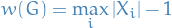
And the treewidth  of a graph is the minimum width among all possible tree decompositions of , i.e.
Stochastic Block Modelling
Notation
- number of vertices, thus
![$v \in [n]$](../../assets/latex/graph_theory_572b16d3a3e596a52b9f6077873ea0d7dff2be40.png)
- number of communities
- n-dimensional random vector with i.i.d. components distributed under
 , i.e. representing the community-assignment of each vertex
  is the random variable representing the community of which vertex belongs to, taking on values in
 ![$[k]$](../../assets/latex/graph_theory_a46760c00adda23a3fc4c4a47e402dee24e8aaad.png) , i.e.
, i.e.  with
with ![$x_v \in [k]$](../../assets/latex/graph_theory_a41b7d71f26a7fe7621f13b84e696f72cfea1448.png)
- is a
 symmetric matrix with vertices and being connected with probability
  , indep. of other pairs of vertices.
 ![$\Omega_i = \Omega_i(X) := \{ v \in [n] \mid X_v = i, i \in [k] \}$](../../assets/latex/graph_theory_88a31b74931296af74a1720cf551c073a7d60381.png) denotes a community set
denotes a community set denotes a community-graph pair
Stuff

- Probability vector of dimension
- Symmetric matrix of dimension with entries in
![$[0, 1]$](../../assets/latex/graph_theory_68c8fa38d960e53d4308cbf1e65d04c66a554817.png)
Then  defines a n-vertex random graph with labelled vertices, where each vertex is assigned a community label in
  independently under the community prior , and pairs of vertices with labels and connect independently with probability
  .
.
Further generalizations allow for labelled edges and continuous vertex labels, conencting to low-rank approximation models and graphons.
Thus the distribution of where ![$G = \big( [n], E(G) \big)$](../../assets/latex/graph_theory_42bccc68275c40f74ab2fd71732bbda541b790e6.png) is
is
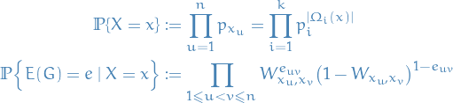
which is just saying:
![\begin{equation*}
\begin{split}
X_u & \sim \text{Multinomial}(k), \quad \forall u \in [n] \\
E_{uv} & \sim \text{Bernoulli}(W_{x_u, x_v}), \quad \forall u, v \in [n], u \ne v
\end{split}
\end{equation*}](../../assets/latex/graph_theory_090207e24f83667a116fe6e96d61c2e989ad2e06.png)
Graphical models
Min-Max propagation
Algorithms
Shortest path
Dijkstra's Shortest Path
And here's a super-inefficient implementation of Djikstra's shortest path algorithm in Python:
import numpy as np
from collections import defaultdict, deque, namedtuple

def is_empty(q):
    return len(q) < 1


def get_neighbors(v, graph):
    neighs = []

    for e in graph.edges:
        if e.vertices[0] == v:
            neighs.append((e, e.vertices[1]))
        elif e.vertices[1] == v:
            neighs.append((e, e.vertices[0]))

    return neighs


# structures
Node = namedtuple('Node', ['value'])
Edge = namedtuple('Edge', ['vertices', 'weight', 'directed'])
Graph = namedtuple('Graph', ['vertices', 'edges'])

# straight foward problem
V = [Node(i) for i in range(10)]
E = [Edge([V[i - 1], V[i]], i, False) for i in range(1, 9)] + [Edge([V[8], V[9]], 0, False)]
G = Graph(V, E)

# shortcut!
E = E + [Edge([V[4], V[8]], -6, False)]
G = Graph(V, E)

v_0 = V[0]   # start
v_n = V[-1]  # stop

paths = {}
path_weights = defaultdict(lambda: np.inf)

seen = set()
queue = deque([v_0, v_n])

seen.add(v_n)

v_curr = queue.popleft()
path_weights[v_curr] = 0 # initialize path weight to 0 from starting point
path_w = path_weights[v_curr]
paths[v_curr] = None

edge, v_neigh = get_neighbors(v_curr, G)[0]
# update best prev vertex candidate for `v_neigh`
paths[v_neigh] = v_curr
# update best candidate weight
path_weights[v_neigh] = edge.weight + path_w

while not is_empty(queue) and v_curr != v_n:
    for (edge, v_neigh) in get_neighbors(v_curr, G):
        if v_neigh == paths[v_curr]:
            # if it's the neighboring vertex we just came from => skip it
            continue

        # proposed path is improvement over previous path with `v_neigh` ?
        candidate_path_weight = path_weights[v_neigh]
        if edge.weight + path_w < candidate_path_weight:
            # update best prev vertex candidate for `v_neigh`
            paths[v_neigh] = v_curr
            # update best candidate weight
            path_weights[v_neigh] = edge.weight + path_w

        if v_neigh not in seen:
            queue.append(v_neigh)
            seen.add(v_neigh)

    # sort `queue` so that the next visit is to the current "shortest" path
    queue = deque(sorted(queue, key=lambda v: path_weights[v]))

    v_curr = queue.popleft()
    path_w = path_weights[v_curr]

# upon termination we simply walk backwards to get the shortest path
optimal_path = [v_n]
v_curr = v_n
while v_curr != v_0:
    v_curr = paths[v_curr]
    optimal_path.append(v_curr)


def display_path(path):
    print("Optimal path: " + " --> ".join([str(v.value) for v in path]))


display_path(list(reversed(optimal_path)))
print("Observe that some nodes are NEVER seen, as we'd like!")

from pprint import pprint
pprint(list(paths.keys()))
Optimal path: 0 --> 1 --> 2 --> 3 --> 4 --> 8 --> 9
Observe that some nodes are NEVER seen, as we'd like!
[Node(value=0),
 Node(value=1),
 Node(value=2),
 Node(value=3),
 Node(value=4),
 Node(value=5),
 Node(value=8),
 Node(value=7),
 Node(value=9)]
#include <iostream>
#include <memory>

template<typename T>
struct BinTreeNode
{
  T value;
  std::shared_ptr<BinTreeNode<T>> left = nullptr;
  std::shared_ptr<BinTreeNode<T>> right = nullptr;

  BinTreeNode(T v) : value(v) { }
};

int main()
{
  std::shared_ptr<BinTreeNode<int>> root = std::shared_ptr<BinTreeNode<int>>(new BinTreeNode<int>(0));
  root->left = std::make_shared<BinTreeNode<int>>(1);
  root->right = std::make_shared<BinTreeNode<int>>(2);

  root->left->left = std::make_shared<BinTreeNode<int>>(4);

  std::cout << root->value << std::endl;
  std::cout << root->left->value << std::endl;
  std::cout << root->left->left->value << std::endl;

  std::shared_ptr<BinTreeNode<int>> current = root;
  for (auto i = 0; i < 10; i++) {
    // using "raw" pointers, these `BinTreeNode` instances will live long enough
    // but risking dangling pointers in the case were we delete a parent node
    // UNLESS we specificly delete them (which we can do using a custom destructor for `BinTreeNode`)

    // Instead we can use `std::shared_ptr` which has an internal reference-counter,
    // deallocating only when there are no references to the object
    std::shared_ptr<BinTreeNode<int>> next = std::make_shared<BinTreeNode<int>>(i);
    std::cout << next->value << std::endl;
    if (next->value >= current->value) {
      current->right = next;
    }
    else {
      current->left = next;
    }

    current = next;
  }

  std::cout << root->right->right->value << std::endl;
  return 0;
}
Bellman-Ford algorithm
- Computes shortest paths from single source vertex to all other vertices in a weighted digraph
- Slower than Dijkstra's Algorithm for same problem, but more versatile
- Capable of handling edges with negative weights
- Can be used to discover negative cycles (i.e. a cycle whose edges sum to a negative value)
- E.g. arbitrage opportunities on Forex markets
Relation to Dijkstra's algorithm:
- Both based on principle of relaxation:
- Approximation of the correct distance is gradually replaced by more accurate values until eventually reaching the optimum solution
- Approx. distnace to each vertex is an overestimate of true distance, and is replacted by the minimum of its old value and the length of the newly found path
- All nodes are initialized to be
 away from the source vertex
  , i.e. an overestimate
 - Update these distances at each iteration
- All nodes are initialized to be
- Difference:
- Dijkstra's: uses priority queue to greedily select the closest vertex that has not been processed, and performs this relaxation process on all of its outgoing edges
- BF: simply relaxes all the edges, and does this
 times (since there can be at most edges on a path between any two vertices)
- Can terminate early if shortest paths does not change between two iterations
- In practive the ordering of which we update the edges can improve the runtime
Impl
def bellman_ford(vertices, edges, source):
    distances = {source: 0.0}
    previous = {}

    # instead of using infinity as initial value, we simply
    # check if the vertex is already in ``distances`` as a
    # proxy for "infinity" distance. Hence we do not need an initialization.

    # perform relaxation iterations
    diff = True
    i = 0

    while diff and i < len(vertices) - 1:
        diff = False

        # iterate over vertices which are reachable
        for v in (v for v in vertices if v in distances):
            v_dist = distances[v]
            outgoing_edges = [e for e in edges if e[0] == v]

            for (_, u, w) in outgoing_edges:
                if u not in distances or v_dist + w < distances[u]:
                    # found new shortert path to vertex ``u``
                    distances[u] = v_dist + w
                    previous[u] = v

                    # made a change
                    diff = True

        # update counter
        i += 1

    return distances


# negative cycle
edges = [
    (0, 1, 1.0),
    (1, 2, 1.0),
    (0, 2, 4.0),
    (2, 3, 1.0),
    (3, 0, -5.0)
]
vertices = [v for v in range(4)]
bellman_ford(vertices, edges, 0)
Conclusion
| Algorithm | Greedy | Negative edges? | Complexity | |
|---|---|---|---|---|
| Dijkstra | Y | N | ||
| Bellman-Ford | N | Y |  |
Code
graph-tool python
import graph_tool.all as gt

g = gt.collection.data["football"]
g
# Out[4]:
: <Graph object, undirected, with 115 vertices and 613 edges at 0x7f25204da438>
state = gt.minimize_blockmodel_dl(g)
state
# Out[6]:
: <BlockState object with 10 blocks (10 nonempty), degree-corrected, for graph <Graph object, undirected, with 115 vertices and 613 edges at 0x7f25204da438>, at 0x7f24d806d588>
_ = state.draw(pos=g.vp.pos, output="./.graph_theory/figures/football-sbm-fit.png")
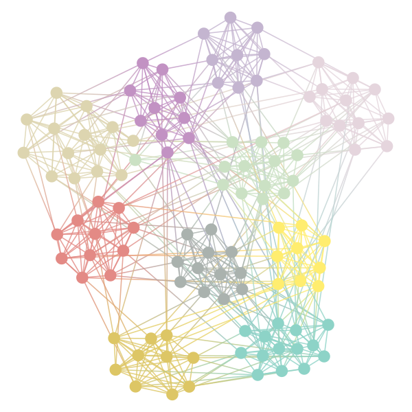
Figure 7: Graph of the football-dataset with the different communities colored.
%matplotlib inline
import matplotlib.pyplot as plt

edges = state.get_matrix()
_ plt.matshow(edges.todense())
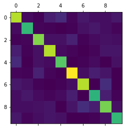
Figure 8: Connections between the different clusters (and the degrees within the clusters along the diagonal)
Course
Notation
Graph is a pair
 where
where  , e.g.

- Order of refers to
 , which is often denoted
- Size of is |E(G)|$, often denoted

- Will only deal with simple graphs (or rather, the def above only includes simple graphs)
 often used to refer to the edge
- If
 we say "
 is adjacent to
  " and might write
Two graphs
 are *isomorphic$ if there exists a bijection
  such that

i.e. edge-preserving bijection between vertices
 is empty graph of order and size 0
 is complete graph of order and size
  , i.e. all pairs vertices adjacent
 is a path of order and size
  is a circuit of order and size , i.e. just a path with the ends joined, or a cycle
- A subgraph of is a graph with
 and
and  (so every graph of order
  is a subgraph of )
 - A subgraph of induced by the subset
 written
 ![$G[W]$](../../assets/latex/graph_theory_f3bb08e5180801458aa10dfc6cf46a9e088d1b95.png) is the graph
is the graph  , i.e. the vector set and all edges of lying inside
Lecture 1
The components of are the maximal connected subgraphs induced by the equivalence classes of the relation "there is a u-v-path or  ".
".
A forest is a graph containing no circuit.
A tree is a connected forest, i.e. components of a forest are trees. Equivalently, it's connected but has no circuit.
The following are equivalent
- is a tree (connected but has no circuit)
- is minimal connected, i.e. is connected but removal of any edge kills connectivity
- is maximial circuit-free, i.e. has no circuit, but addition of any new edge creates a circuit
 : Let be connected circuit free. Suppose
  and
and  is connected (i.e. without the edge
  ). Then there is a path
  in , so contains the circuit
  . Thus contradiction means is minimal connected.
 : Let be minimal conected. Suppose has a circuit and let
  . Then,
  and
and  are connected by at least two paths, so we can remove one edge along one of these paths but still remain connected
  is circuit-free.
 : Let be a tree. If
  there is a path in from to , so is a circuit in
  . So is maximal circuit-free.
 : Let be maximal circuit-free. Let . Either
  or has a circuit so
  is a u-v-path in . Either way is joined to , so is connected.
Discrete Exterior Calculus
- Great quick overview of the idea: http://www.cs.jhu.edu/~misha/Fall09/17-dec.pdf
- Based on a set of notes which looks really promising: desbrun05_discr_exter_calcul