Theory
Table of Contents
Overview
This document covers a lot of the more "pure" sides of Machine Learning, e.g. attempts at establishing bounds on convergence.
Most of this is built upon the Probably Approximately Correct (PAC) framework, which attempts to bound the errors the generalization of models.
Good sources, where I've gotten a lot of this from:
Notation
![$[m] = \left\{ 1, \dots, m \right\}$](../../assets/latex/theory_e48738a920711d373ed16fd09958ff87095e9692.png) , for a
, for a 
 denotes the result of applying
  to
to  ,
,
 denotes the true risk of
  , where
  is the distribution, and
  the labelling-function
 denotes denotes the probability of getting a nonrepresentative sample, and we say
  is the confidence parameter of our prediction
 denotes the accuracy parameter, dealing with the fact that we cannot guarantee perfect label prediction:
  is a failure of the learner, while
  means we view the output of the learner as approximately correct
 denotes an instance of the training set
Empirical Risk Minimization rule is denoted:
i.e. the set of learners which minimizes the empirical risk
 .
.
bb* Empirical Risk Minimization (EMR) Standard Empirical Risk Minimization: minimize the empirical loss
![\begin{equation*}
L_S(h) = \frac{\big| i \in [m] : h(x_i) \ne y_i \big|}{m}
\end{equation*}](../../assets/latex/theory_74e054325d90d9d067186062e0163ec406f7dcd4.png)
A risk function is the expected loss of classifier  wrt. the probability distribution over
  , namely
![\begin{equation*}
L_{\mathcal{D}}(h) := \mathbb{E}_{z \sim \mathcal{D}} \big[ \ell(h, z) \big]
\end{equation*}](../../assets/latex/theory_29844aa82ccf60f88e7bd1990968e7e911ffb140.png)
Empirical risk is the expected loss over a given sample  , namely,
Finite Hypothesis Classes
- Simple restriction in attempt to avoid "overfitting" is to bound the size of the hypotheses; i.e. consider a restricted hypothesis class

For now we make the following assumption:
There exists  such that
That is, there exists an optimal hypothesis in the restricted hypothesis class which obtaines the global minimum true risk, i.e. minimum loss over the full data distribution.
Hence, we would like to upper bound the probability to sample m-tuple of instances which lead to failure. That is, find an upper bound for
Then let
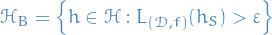
i.e. all the "bad" hypotheses, such that the probability of failure of the learner is greater than .
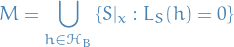
Further, let

i.e.  is set of all training instances which would "mislead" us into believing one of the wrong hypotheses (
 ) is "good" (i.e. has zero average loss on the training data).
With our Realizability Assumption (i.e. that  ), then

can only happen if for some we have  . That is,

which means that

Further, we can rewrite
Hence,

To summarize: probability of learner failing in an sense, is bounded above by the probability of the learner being a misleading learner, i.e. having minimal training error and being in the "bad" hypotheses class.
And because of how probability-measures work, probabilities of finite unions can be written

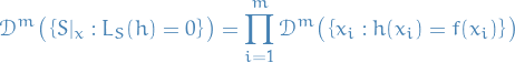
Suppose now that . By definition,
![\begin{equation*}
L_S(h) = 0 \iff h(x_i) = f(x_i), \quad \forall i \in [m]
\end{equation*}](../../assets/latex/theory_b3758f6f4d9f1cad2d3084269620aeea0b207656.png)
and due to the i.i.d. sampling of the training set, the joint probability of this occuring is then
Further, for each individual sample in the training set we have

where the last inequality follows from the fact that .

simply denotes the probability of this correctly labelling the  over the entire true distribution . Since these equalities are indicator variables, thus binary, this corresponds to the expectation
![\begin{equation*}
\mathbb{E} \big[ h(x) = y \big]
\end{equation*}](../../assets/latex/theory_aad9a2c6302bdd5b3ce6249f854b3daefd6c396a.png)
and since ![$L_{(\mathcal{D}, f)}(h) = \mathbb{E}[h(x) \ne y]$](../../assets/latex/theory_0036225e85859650509a9ed460eb7d4ae280a843.png) by definition, we have
by definition, we have

which is the second equality in the above expression.
Finally, observing that for  , we have

we obtain

Combining this with the sum over the we saw earlier, we conclude that

Let
- be a finite hypothesis class

- such that
Then, for any labeling function , and any distribution , for which the realizability assumption holds, over the choice of an i.i.d. sample of size  , we have that for every ERM hypothesis, ,

That is, the rule over a finite hypothesis class will be probably (with confidence  ) approximately (up to error ) correct (PAC).
Probably Approximately Correct (PAC)
A hypothesis class is PAC learnable if there exist a function  and a learning algorithm with the property:
- for every

- for every distribution over

- for every labeling function
if the realizable assumption holds wrt. , , and , then when running the learning algorithm on  i.i.d. examples generated by and labeled by , the algorithm returns a hypothesis
  s.t.
s.t.

We will often refer to  as the sample complexity of learning .
- defines how far the output classifier can be from the optimal one
- is how likely the classifier is to meet the accuracy requirement
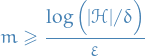
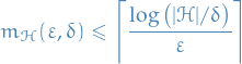
Every finite hypothesis class is PAC learnable with sample complexity
Agnostic PAC learning - relaxing realization assumption
A hypothesis class is agnostic PAC learnable wrt a set and a loss function  , if there exists a function and an algorithm with the property
- for every
- for every distribution over
when running the learning algorithm on i.i.d. examples drawn from , the algorithm returns such that

where
![\begin{equation*}
L_{\mathcal{D}}(h) = \underset{z \sim \mathcal{D}}{\mathbb{E}} \big[ \ell(h, z) \big]
\end{equation*}](../../assets/latex/theory_c4c6df9e2a99745e926ee1c19a74fe9174625abb.png)
Uniform convergence
A training sample is called  wrt. domain , hypothesis class , loss function
  , and distribution , if

Assume that a training set is  .
.
Then, any output of  , namely, any
satisfies
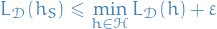
From Lemma 4.2 we know that a  rule is an agnostic PAC-learner if is with probability !
This is motivates the following definition of Uniform Convergence:
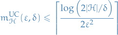
We say that a hypothesis class has the uniform convergence property (wrt. domain and loss ) if there exists a function  such that for
- every
- every probability distribution over
if is a sample of  examples drawn i.i.d. according to , then is , with at least probability .
Let  be a sequence of i.i.d. random variables and assume that for all i,
![\begin{equation*}
\mathbb{E}[\theta_i] = \mu, \quad \mathbb{P} \big[ a \le \theta_i \le b \big] = 1
\end{equation*}](../../assets/latex/theory_8cb0ab9601c74549e2157fdd6800c0b65e0164b9.png)
Then, for any ,
![\begin{equation*}
\mathbb{P} \Bigg[ \frac{1}{m} \left| \sum_{i=1}^{m} \theta_i - \mu \right| > \varepsilon \Bigg] \le 2 \exp \Big( - 2 m \varepsilon^2 / (b - a)^2 \Big)
\end{equation*}](../../assets/latex/theory_13cdda5683d593ca656e7a65bed422892021a6ae.png)
Using Hoeffding's Inequality, one can prove the following:
Let be a finite hypothesis class, let be a domain, and let ![$\ell: \mathcal{H} \times Z \to [0, 1]$](../../assets/latex/theory_bc182736c1681a336f1d30dfefbee990980ad370.png) be a loss function.
be a loss function.
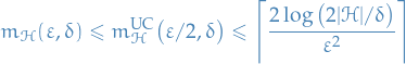
Then, enjoys the uniform convergence property with sample complexity
Furthermore, the class is agnostically PAC learnable using the ERM algorithm with sample complexity
Even though Corollary 4.6 only holds for finite hypothesis in practice it might also provide us with upper bounds to "infinite" hypothesis classes, due to parameters most often being represented using floating point representations, which consists of 64 bits.
That is, if we're computationally approximating some  , there is only
  different values
  actually can take on. If we then have
  parameters, we can use Corollary 4.6 to obtain the following bound:
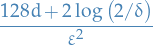
This is often referred to as the discretization trick.
Bias-Complexity Tradeoff
Let  be any learning algorithm for the task of binary classification wrt. to the 0-1 loss over a domain .
Let be any number smaller than
be any learning algorithm for the task of binary classification wrt. to the 0-1 loss over a domain .
Let be any number smaller than  , representing a training set size.
Then, there exists a distribution over  such that:
- There exists a function
 with
with 
With probability of at least
 over the choice of
  we have that
No-Free-Lunch theorem states that for every learner, there exists a task on which it fails even though that task can be successfully learned by another learner.
Let  such that
  .
.
We will prove this using the following intuition:
- Any learning algorithm that observes only half of the instances in
 has no information on what should be the labels of the rest of the instances in
 - Therefore, there exists a "reality", that is some target function , that would contradict the labels that
 predicts on the unobserved instances in
Since by assumption, there are  unique mappings
  . Denote these
  . For each
  , let
, let  be a distribution over
  defined by
Then we have

We can combine Lemma lemma:no-free-lunch-theorem-intermediate-lemma-1 with Lemma lemma:shalev2014understanding-B1, from which we observe
![\begin{equation*}
\mathbb{P} \big[ Z > 1 / 8 \big] \ge \frac{\mu - 1 / 8}{1 - 1 / 8} = \frac{\mu - 1 / 8}{7 / 8} = \frac{8}{7} \mu - \frac{1}{7} \ge \frac{8}{7} \cdot \frac{1}{4} - \frac{1}{7} = \frac{2}{7} - \frac{1}{7} = \frac{1}{7}
\end{equation*}](../../assets/latex/theory_99828d111f908678e499221c45fb63f2f9d1915f.png)
where we've used ![$\mu = \mathbb{E} \big[ L_{\mathcal{D}} \big( A(S) \big) \big] \ge \frac{1}{4}$](../../assets/latex/theory_0f884bc814a935b8e8c0d7cd66938e9007c24c74.png) . Hence,
. Hence,
![\begin{equation*}
\mathbb{P} \big[ Z > 1 / 8 \big] \ge \frac{1}{7}
\end{equation*}](../../assets/latex/theory_19525aa0d12d16d7f02eed077b99223ceac0d2e4.png)
concluding our proof.
For every algorithm  , that receives a training set of examples from there exists a function and a distribution over , such that and
![\begin{equation*}
\underset{S \sim D^m}{\mathbb{E}} \big[ L_{\mathcal{D}} \big( A(S) \big) \big] \ge \frac{1}{4}
\end{equation*}](../../assets/latex/theory_a1c4e7f382321f7d66dcaf658da5870106a494a2.png)
Let be some algorithm that receives a training set of examples from and returns a function  , i.e.
There are  possible sequences of samples from . Let
and
i.e.  denotes the sequences containing instances in
  labeled by .
If the distribution is , as defined above, then the possible training sets can receive are  , and all these training sets have the same probability of being sampled. Therefore,
![\begin{equation*}
\underset{S \sim \mathcal{D}_i^m}{\mathbb{E}} \big[ L_{\mathcal{D}_i} \big( A(S) \big) \big] = \frac{1}{k} \sum_{j=1}^{k} L_{\mathcal{D}_i} \big( A(S_j^i) \big)
\end{equation*}](../../assets/latex/theory_54c15d0e007a14b378c209842fc6c637edc0fc95.png)
Using the fact that maximum is larger than average, and average is larger than minimum, we have
![\begin{equation*}
\begin{split}
\max_{i \in [T]} \frac{1}{k} \sum_{j=1}^{k} L_{\mathcal{D}_i} \big( A(S_j^i) \big)
& \ge \frac{1}{T} \sum_{i=1}^{T} \frac{1}{k} \sum_{j=1}^{k} L_{\mathcal{D}_i} \big( A(S_j^i) \big) \\
&= \frac{1}{k} \sum_{j=1}^{k} \frac{1}{T} \sum_{i=1}^{T} L_{\mathcal{D}_i} \big( A(S_j^i) \big) \\
& \ge \min_{j \in [k]} \frac{1}{T} \sum_{i=1}^{T} L_{\mathcal{D}_i} \big( A(S_j^i) \big)
\end{split}
\end{equation*}](../../assets/latex/theory_9c33a8e69751300944324af64bf4bb90a2cbd088.png)
The above equation is saying that the maximum risk expected over possible rearrangements of achieved by  is greater than the minimum of the expected risk over possible using the optimal arrangement ordering of .
Now, fix some ![$j \in [k]$](../../assets/latex/theory_e747e9c4bf21f864dade19712be4f9737aba2dfc.png) , and denote
, and denote  and let
  be the examples in that do not appear in , i.e.
![\begin{equation*}
v_a : v_a \ne x_b, \quad \forall b \in [m], \quad \forall a \in [p]
\end{equation*}](../../assets/latex/theory_503415d205068bcf09fab029494e338c8ebb50ad.png)
Clearly  , since we're assuming and
  , and therefore the "best" case scenario is if we get distinct samples.
Therefore, for every function  and every
 ![$i \in [T]$](../../assets/latex/theory_2b7ffbfdd966e63b901eb26d45b24c63addbb938.png) we have
we have
![\begin{equation*}
\begin{split}
L_{\mathcal{D}_i}(h) &= \frac{1}{2m} \sum_{x \in C}^{} \mathbbm{1} \big[ h(x) \ne f_i(x) \big] \\
&\ge \frac{1}{2m} \sum_{r=1}^{p} \mathbbm{1} \big[ h(v_r) \ne f_i(v_r) \big] \\
&\ge \frac{1}{2p} \sum_{r=1}^{p} \mathbbm{1} \big[ h(v_r) \ne f_i(v_r) \big]
\end{split}
\end{equation*}](../../assets/latex/theory_89d4504df8478e45b5ad0f75553930d365522496.png)
Hence,
![\begin{equation*}
\begin{split}
\frac{1}{T} \sum_{i=1}^{T} L_{\mathcal{D}_i} \Big( A(S_j^i) \Big)
& \ge \frac{1}{T} \sum_{i=1}^{T} \frac{1}{2p} \sum_{r=1}^{p} \mathbbm{1} \big[ A(S_j^i)(v_r) \ne f_i(v_r) \big] \\
& = \frac{1}{2p} \sum_{r=1}^{p} \frac{1}{T} \sum_{i=1}^{T} \mathbbm{1} \big[ A(S_j^i)(v_r) \ne f_i(v_r) \big] \\
&\ge \frac{1}{2} \min_{r \in [p]} \frac{1}{T} \sum_{i=1}^{T} \mathbbm{1} \big[ A(S_j^i)(v_r) \ne f_i(v_r) \big]
\end{split}
\end{equation*}](../../assets/latex/theory_837c0656c73067f8c03f39b4131a8517d0623cb0.png)
Next, fix some ![$r \in [p]$](../../assets/latex/theory_af9cabe0b509536fa1e8dd275c59c10895690fd9.png) .
.
We can partition all the functions in into  disjoint pairs, where for a pair
  we have

Since such a pair must have  , it follows that
![\begin{equation*}
\mathbbm{1} \big[ A(S_j^i)(v_r) \ne f_i(v_r) \big] + \mathbbm{1} \big[ A(S_j^{i'})(v_r) \ne f_i(v_r) \big] = 1
\end{equation*}](../../assets/latex/theory_db3b3acb6a83d70a8cb70922d42a1f9e75e8e7e3.png)
which yields
![\begin{equation*}
\frac{1}{T} \sum_{i=1}^{T} \mathbbm{1} \big[ A(S_j^i)(v_r) \ne f_i(v_r) \big] = \frac{1}{2}
\end{equation*}](../../assets/latex/theory_26129d3eaaff46597e6d6f2219ed18ff8cdff17b.png)
Substituting this back into
![\begin{equation*}
\frac{1}{T} \sum_{i=1}^{T} L_{\mathcal{D}_i} \Big( A(S_j^i) \Big) \ge \frac{1}{2} \min_{r \in [p]} \frac{1}{T} \sum_{i=1}^{T} \mathbbm{1} \big[ A(S_j^i)(v_r) \ne f_i(v_r) \big] = \frac{1}{4}
\end{equation*}](../../assets/latex/theory_9cc600295632d0c840acd933a3c30bfd4192d79a.png)
and this into
![\begin{equation*}
\max_{i \in [T]} \underset{S \sim \mathcal{D}_i^m}{\mathbb{E}} \big[ L_{\mathcal{D}_i} \big( A(S_j^i) \big) \big] \ge \max_{i \in [T]} \frac{1}{k} \sum_{j=1}^{k} L_{\mathcal{D}_i} \big( A(S_j^i) \big) \ge \frac{1}{T} \sum_{i=1}^{T} L_{\mathcal{D}_i} \big( A(S_j^i) \big) \ge \frac{1}{4}
\end{equation*}](../../assets/latex/theory_ac6452828388149bad7ea23298433af7ed9253a3.png)
Hence, there exists a sample such that
![\begin{equation*}
\underset{S \sim \mathcal{D}^m}{\mathbb{E}} \Big[ L_{\mathcal{D}} \big( A'(S) \big) \Big] \ge \frac{1}{4}
\end{equation*}](../../assets/latex/theory_aa71d53738c4bca50b58a3bbc6b9635aa73fd476.png)
for every algorithm .
We decompose the error of an  predictor into two components as follows.
Let be an hypothesis. Then, we can write

where

 denotes the approximation error, which is the minimum possible risk achievable by a predictor in the given hypothesis class
  denotes the estimation error, which is the difference between the best achivable error and the error achieved by
The VC-Dimension
Let be a class of functions from to  , and let
  .
.
The restriction of to is the set of functions which can be derived from . That is,
A hypothesis class shatters a finite set if the restriction of to is the set of all functions .
That is, if  .
.
Shattering is basically a way of stating
- All functions mapping from the subset to the set of binary labels
- If the hypothesis-class we're trying to learn contains all possible functions from to then we say it's shattered, and this indicates that it will be difficult (if not impossible) to learn due to the fact that if
 and is shattered by , i.e.
  is the set of all possible mappings
  , then is not PAC-learnable, since we cannot satisfy arbitrary bounds simply by adjusting the number of samples.
The VC-dimension of a hypothesis class denoted  , is the maximal size of a set that can be shattered by .
If can shatter sets of arbitrarily large size, we say that has infinite VC-dimension.
Let be a class of infinite VC-dimension. Then, is not PAC-learnable.
Generalization
Here we will consider generalization on classification tasks using PAC-learning theory.
Notation
 samples of inputs and outputs
 distribution on labelled data
 denotes i.i.d. samples of data bpoints
  from (often just write , and have the be implied)
- denotes the set of classifiers / hypotheses which we consider to explain the data
 denotes the loss of classifier on point
 denotes the average loss of classifier on the sample-set
  , i.e.
![\begin{equation*}
L_{S_m}(h) = \mathbb{E}_{z \sim S_m} \big[ l(h, z) \big]
\end{equation*}](../../assets/latex/theory_d864767f037ebaa9e2bee726499f0435dd228e35.png)
 denotes the average loss over the entire distribution :
![\begin{equation*}
L_D(h) = \mathbb{E}_{z \sim D} \big[ l(h, z) \big]
\end{equation*}](../../assets/latex/theory_2d2eaec18723189c27918935071b169b0d483c36.png)
Generalization error

Generalization under ERM
The objective is
i.e. which best explains the dataset, which is Empirical Risk Minimization since we're minimizing the empirical loss.
We then define the generalization error as follows:
The generalization error is defined
which measures how well hypothesis generalizes to a distribution when its performance on a sample drawn from is known.
Generalization Theory
- Generalization theory attempts to upper bound the
 from the generalization error
Rademacher Complexity
- Formalize notion of complexity of a hypothesis
Let
- is the hypothesis class
- is
 i.i.d. samples from
 And then the coefficients
Then the Rademacher Complexity of on a distribution is defined as
![\begin{equation*}
\mathcal{R}_{m, D}(\mathcal{H}}) = \underset{S \sim D^m}{\mathbb{E}} \Bigg[ \frac{1}{2m} \sup_{h \in \mathcal{H}} \Big| \sum_{i=1}^{2m} \sigma_i h(z_i) \Big| \Bigg]
\end{equation*}](../../assets/latex/theory_24f2a36b15f5a91fd190668d0d239988b2208b41.png)
The  simply flip the sign of the classification (we're assuming
  for all
  ) simply changes the classification of to opposite one.
This therefore corresponds to flipping the labels of half the datapoints randomly and retaining the labels of the other half. We choose the which correlates well with this random relabeling (if half classified as positive and half classified as negative, and then for this specific we just happen to flip all the the ones which are positive to negative, then we get our  ).
).
I struggle a bit with interpreting the Rademacher Complexity intuitively. Why would this indicate high complexity of the hypothesis class?
- Because we can consider ….
For a given loss function , we have that the generalization error of all hypothesis on a sample of i.i.d. samples drawn from a distribution , is
for all  , with probability
  .
.
Hence, the generalization error of a hypothesis can be upper bounded by the Rademacher complexity.
This is more a sketch of the poof.
Suppose for a random sample the generalization error is high. Then
- Split into sets
 and
and  randomly, with sets being of equal size
 - For a given (picked independently of ), consider
 and
and 
For large
, we have  and thus

(with
being sort of like our "test" set and the "training" set). Thus
Since
and are picked randomly, we can just consider as the first half of the samples and then the difference reduces to
![\begin{equation*}
\begin{split}
\underset{S \sim D^m}{\mathbb{E}} \Bigg[ \underset{z \sim S_2}{\mathbb{E}} \big[ L(h, z) \big] - \underset{z \sim S_1}{\mathbb{E}} \big[ L(h, z) \big] \Bigg]
&\le \underset{S \sim D^m}{\mathbb{E}} \Bigg[ \frac{1}{m} \Big| \sum_{i=1}^{m} \sigma_i h_i(z_i) \Big| \Bigg] \\
& \le \sup_{h \in \mathcal{H}} \underset{S \sim D^m}{\mathbb{E}} \Bigg[ \frac{1}{m} \Big| \sum_{i=1}^{m} \sigma_i h(z_i) \Big| \Bigg]
\end{split}
\end{equation*}](../../assets/latex/theory_fe018defdb8934ceaa73642e1611b9cdf66258dc.png)
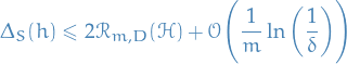
Thus we have
![\begin{equation*}
\begin{split}
\Delta_S(h) & \le \sup_{h \in \mathcal{H}} \underset{S \sim D^m}{\mathbb{E}} \Bigg[ \Big| \frac{1}{m} \sum_{i=1}^{m} \sigma_i h(z_i) \Big| \Bigg] \\
& \le \underset{S \sim D^m}{ \mathbb{E}} \Bigg[ \sup_{h \in \mathcal{H}} \frac{1}{m} \Big| \sum_{i=1}^{m} \sigma_i h(z_i) \Big| \Bigg] = 2 \mathcal{R}_{m, D}(\mathcal{H})
\end{split}
\end{equation*}](../../assets/latex/theory_e7a7026f7b7bc9ee56f24bdd3e81e49f2aca981a.png)
where the factor of
 is simply due to our definition of Rademacher complexity involving .
We also leave out the "concentration term" (I believe this depends on the "variance" of the underlying distribution)
is simply due to our definition of Rademacher complexity involving .
We also leave out the "concentration term" (I believe this depends on the "variance" of the underlying distribution)
Let
 be a sequence of independent random variables taking on values in a set
  be a sequence of positive real constants
If  satisfies

for  , then
![\begin{equation*}
\mathbb{P} \big( \left\{ \varphi(z_1, \dots, z_m) - \mathbb{E}_{z_1, \dots, z_m} \big[ \varphi(z_1, \dots, z_m) \big] \right\} \ge \varepsilon \big) \le \exp \bigg( - \frac{2 \varepsilon^2}{\sum_{i=1}^{n} c_i^2} \bigg)
\end{equation*}](../../assets/latex/theory_e07a5b5139b94c8570bac7e484c5d01aec88de38.png)
Let
- be a fixed distribution over the space
- be a given constant
 be a set of bounded functions, wlog. we in particular assume
 ![$\mathcal{F} \subseteq \left\{ f: Z \to [0, 1] \right\}$](../../assets/latex/theory_b9b00a1f655c36361ead9aae84eefee57fde4236.png)
 be a sequence of i.i.d. samples from
Then, with probability at least over the draw of , for every function  ,
,
![\begin{equation*}
\mathbb{E}_D \big[ f(z) \big] \le \widehat{\mathbb{E}}_S \big[ f(z) \big] + 2 R_m(\mathcal{F}) + \sqrt{\frac{\log (1 / \delta)}{m}}
\end{equation*}](../../assets/latex/theory_a655ec27a00c1747ff46e12ccc36c29cf89898be.png)
We have
![\begin{equation*}
\mathbb{E}_D \big[ f(z) \big] - \widehat{\mathbb{E}}_S \big[ f(z) \big] \le \sup_{h \in \mathcal{F}} \bigg( \mathbb{E}_D \big[ h(z) \big] - \widehat{\mathbb{E}}_S \big[ h(z) \big] \bigg)
\end{equation*}](../../assets/latex/theory_84daf4a8bc90fb07b1c4aab73fda6289e8cc3ac2.png)
so
![\begin{equation*}
\mathbb{E}_D \big[ f(z) \big] \le \widehat{\mathbb{E}}_S \big[ f(z) \big] + \sup_{h \in \mathcal{F}} \bigg( \mathbb{E}_D \big[ h(z) \big] - \widehat{\mathbb{E}}_S \big[ h(z) \big] \bigg)
\end{equation*}](../../assets/latex/theory_db38593444cbdefaf28694012b4389db933392c3.png)
Consider letting
![\begin{equation*}
\varphi(S) = \sup_{h \in \mathcal{F}} \mathbb{E}_D \big[ h(z) \big] - \widehat{\mathbb{E}}_S \big[ h(z) \big]
\end{equation*}](../../assets/latex/theory_341e02b0cc9855b2d7325d310943944d11d475cd.png)
Let  with
with  being identitically distributed as . Then
![\begin{equation*}
\left| \varphi \big( S \big) - \varphi \big( \tilde{S}_i \big) \right| = \left| \widehat{\mathbb{E}}_{S} \big[ h(z) \big] - \widehat{\mathbb{E}}_{\tilde{S}_i} \big[ h(z) \big] \right| = \frac{1}{m} \sup_{h \in \mathcal{F}} \left| h(z_i) - h(\tilde{z}_i) \right|
\end{equation*}](../../assets/latex/theory_6c7ad988ae7e5f3ff1468f787ba05d33a0e5fed3.png)
and, finally, since are bounded and we assume are all bounded, we can wlog. assume
Thus,
Using McDarmid's inequality, this implies that
![\begin{equation*}
\mathbb{P} \big( \varphi(S) - \mathbb{E}_S \big[ \varphi(S) \big] \ge t \big) \le e^{- t^2 / \big( \frac{1}{m} \sum_{i=1}^{m} \frac{1}{m^2} \big)} = e^{- t^2 m}
\end{equation*}](../../assets/latex/theory_72bda96b07f0b30a1f7a70cbe508f2120f1dce22.png)
One issue: don't yet know how to compute ![$\mathbb{E} [ \varphi(S) ]$](../../assets/latex/theory_c7d1727fd9c48b56934ea441bfd80065ecdc0331.png) !
!
First let's solve for  such that the above probability is
  :
:
And since
![\begin{equation*}
\mathbb{P} \Big( \left\{ \varphi(S) - \mathbb{E}_S[\varphi(S)] \le t \right\} \Big) = 1 - \mathbb{P} \Big( \left\{ \varphi(S) - \mathbb{E}_S \big[ \varphi(S) \big] \ge t \right\} \Big) \ge 1 - \delta
\end{equation*}](../../assets/latex/theory_5771eb8287a2e11588256d14e1f3ab4dec25015d.png)
which is what we want. Thus, with probability at least , we have deduced that
![\begin{equation*}
\varphi(S) \le \mathbb{E}_S \big[ \varphi(S) \big] + \underbrace{\sqrt{\frac{\log(1 / \delta)}{m}}}_{t}
\end{equation*}](../../assets/latex/theory_7840784d87c955584e08bd850bff99b1a059352d.png)
and thus, substituting into our original bound on ![$\mathbb{E}_D \big[ f(z) \big]$](../../assets/latex/theory_d0297aeb185fe32963d68707b0d06938fe94f7c3.png) ,
,
![\begin{equation*}
\begin{split}
\mathbb{E}_D \big[ f(z) \big] &= \widehat{\mathbb{E}}_S \big[ f(z) \big] + \sup_{h \in \mathcal{F}} \bigg( \mathbb{E}_D \big[ h(z) \big] - \widehat{\mathbb{E}}_S \big[ h(z) \big] \bigg) \\
&= \widehat{\mathbb{E}}_S \big[ f(z) \big] + \varphi(S) \\
&\le \widehat{\mathbb{E}}_S \big[ f(z) \big] + \mathbb{E}_S \big[ \varphi(S) \big] + \sqrt{\frac{\log(1 / \delta)}{m}} \\
&= \widehat{\mathbb{E}}_S \big[ f(z) \big] + \mathbb{E}_S \Bigg[ \sup_{h \in \mathcal{F}} \bigg( \mathbb{E}_D\big[h(z)\big] - \widehat{\mathbb{E}}_S \big[h(z)\big] \bigg) \Bigg] + \sqrt{\frac{\log(1 / \delta)}{m}}
\end{split}
\end{equation*}](../../assets/latex/theory_dffd2c12fed70a47159ec08c72b43fc7579c1d4f.png)
with probability at least .
We're now going to make use of a classic symmetrization technique. Observe that due to the independence of the samples
![\begin{equation*}
\mathbb{E}_{\tilde{S}} \Big[ \widehat{\mathbb{E}}_{\tilde{S}} \big[ h(z) \big] \mid S \Big] = \frac{1}{m} \sum_{i=1}^{m} \underbrace{\mathbb{E}_{\tilde{S}} \big[ h(\tilde{z}_i) \mid S \big]}_{= \mathbb{E}_D [ h(z)]} = \frac{1}{m} \sum_{i=1}^{m} \mathbb{E}_D \big[h(z) \big] = \mathbb{E}_D \big[ h(z) \big]
\end{equation*}](../../assets/latex/theory_d333df714ae9c2d3617e96ed255c177bfa815ec6.png)
and
![\begin{equation*}
\mathbb{E}_{\tilde{S}} \Big[ \widehat{\mathbb{E}}_S \big[ h(z) \big] \mid S \Big] = \widehat{\mathbb{E}}_S \big[ h(z) \big]
\end{equation*}](../../assets/latex/theory_53fed5ac59704b268231cbe76202c62c355deef9.png)
The reason why we're writing ![$\mathbb{E}_{\tilde{S}} \big[ \hat{\mathbb{E}}_S[h(z)] \mid S \big]$](../../assets/latex/theory_2d83569a498549c417814749235c3f3ef1019ff2.png) rather than just
rather than just ![$\mathbb{E}_{\tilde{S}} \big[ \hat{\mathbb{E}}_S[h(z)] \big]$](../../assets/latex/theory_234dd6e14ed192c0eb666ca6d40d47ee138ff793.png) is because, if we're being rigorous, we're really taking the expectation over the 2m-dimensional product-space.
is because, if we're being rigorous, we're really taking the expectation over the 2m-dimensional product-space.
Therefore, we can write
![\begin{equation*}
\begin{split}
\mathbb{E}_S \Bigg[ \sup_{h \in \mathcal{F}} \bigg( \mathbb{E}_D \big[ h(z) \big] - \widehat{\mathbb{E}}_S \big[ h(z) \big] \bigg) \Bigg] &= \mathbb{E}_S \Bigg[ \sup_{h \in \mathcal{F}} \bigg( \mathbb{E}_{\tilde{S}} \Big[ \widehat{\mathbb{E}}_{\tilde{S}} \big[ h(z) \big] \mid S \Big] - \mathbb{E}_{\tilde{S}} \Big[ \widehat{\mathbb{E}}_S \big[ h(z) \big] \Big] \bigg) \Bigg] \\
&= \mathbb{E}_S \Bigg[ \sup_{h \in \mathcal{F}} \bigg( \mathbb{E}_{\tilde{S}} \Big[ \widehat{\mathbb{E}}_{\tilde{S}} \big[ h(z) \big] - \widehat{\mathbb{E}}_S \big[ h(z) \big] \mid S \Big] \bigg) \Bigg]
\end{split}
\end{equation*}](../../assets/latex/theory_718393a114422f73230338436d805530f5cb7d80.png)
Moreover, we can use the fact that is a convex function, therefore Jensen's inequality tells us that
![\begin{equation*}
\begin{split}
\mathbb{E}_S \Bigg[ \sup_{h \in \mathcal{F}} \bigg( \mathbb{E}_{\tilde{S}} \Big[ \widehat{\mathbb{E}}_{\tilde{S}} \big[ h(z) \big] - \widehat{\mathbb{E}}_S \big[ h(z) \big] \mid S \Big] \bigg) \Bigg]
&\le \mathbb{E}_S \bigg[ \mathbb{E}_{\tilde{S}} \Big[ \sup_{h \in \mathcal{F}} \Big( \widehat{\mathbb{E}}_{\tilde{S}} \big[ h(z) \big] - \widehat{\mathbb{E}}_S \big[ h(z) \big] \Big) \mid S \Big] \bigg] \\
&= \mathbb{E}_{S, \tilde{S}} \bigg[ \sup_{h \in \mathcal{F}} \bigg( \Big[ \widehat{\mathbb{E}}_{\tilde{S}} \big[ h(z) \big] - \widehat{\mathbb{E}}_S \big[ h(z) \big] \Big] \bigg) \bigg]
\end{split}
\end{equation*}](../../assets/latex/theory_d3aaf6a4ae081c77bd2e212e277393703d6cab8e.png)
Since
![\begin{equation*}
\widehat{\mathbb{E}}_{\tilde{S}} \big[ h(z) \big] - \widehat{\mathbb{E}}_S \big[ h(z) \big] = \frac{1}{m} \sum_{i=1}^{m} \big( h(\tilde{z}_i) - h(z_i) \big)
\end{equation*}](../../assets/latex/theory_840db1d6c6ec177a24db73d3b18015bff58be371.png)
the above is then
![\begin{equation*}
\mathbb{E}_S \Bigg[ \sup_{h \in \mathcal{F}} \bigg( \mathbb{E}_{\tilde{S}} \Big[ \widehat{\mathbb{E}}_{\tilde{S}} \big[ h(z) \big] - \widehat{\mathbb{E}}_S \big[ h(z) \big] \mid S \Big] \bigg) \Bigg] \le \mathbb{E}_{S, \tilde{S}} \Bigg[ \sup_{h \in \mathcal{F}} \bigg( \frac{1}{m} \sum_{i=1}^{m} \Big( h(\tilde{z}_i) - h(z_i) \Big) \bigg) \Bigg]
\end{equation*}](../../assets/latex/theory_43e86ab4ce6def6742fcc3d61f156396f6e5cd6a.png)
This is where the famous Rademacher random variables  , with probability
  , come in: note that
![\begin{equation*}
\mathbb{E}_{\sigma, \mathcal{D}} \big[ \sigma f(z) \big] = \mathbb{E}_D \big[ f(z) \big]
\end{equation*}](../../assets/latex/theory_e0f9472b0e7d6d570b91d61dca18c96d7800e265.png)
for any integrable function . In particular,
![\begin{equation*}
\begin{split}
\mathbb{E}_{S, \tilde{S}} \Bigg[ \sup_{h \in \mathcal{F}} \bigg( \frac{1}{m} \sum_{i=1}^{m} \Big( h(\tilde{z}_i) - h(z_i) \Big) \bigg) \Bigg]
&= \mathbb{E}_{S, \tilde{S}, \sigma} \Bigg[ \sup_{h \in \mathcal{F}} \bigg( \frac{1}{m} \sum_{i=1}^{m} \sigma_i \Big( h(\tilde{z}_i) - h(z_i) \Big) \bigg) \Bigg] \\
&= \mathbb{E}_{S, \tilde{S}, \sigma} \Bigg[ \sup_{h \in \mathcal{F}} \bigg( \frac{1}{m} \sum_{i=1}^{m} \sigma_i h(\tilde{z}_i) + \frac{1}{m} \sum_{i=1}^{m} (- \sigma_i) h(z_i) \bigg) \Bigg] \\
&\le \mathbb{E}_{S, \tilde{S}, \sigma} \Bigg[ \sup_{h \in \mathcal{F}} \bigg( \frac{1}{m} \sum_{i=1}^{m} \sigma_i h(\tilde{z}_i) \bigg) + \sup_{h \in \mathcal{F}} \bigg( \frac{1}{m} \sum_{i=1}^{m} \sigma_i h(z_i) \bigg) \Bigg] \\
&= \mathbb{E}_{\tilde{S}, \sigma} \Bigg[ \sup_{h \in \mathcal{F}} \bigg( \frac{1}{m} \sum_{i=1}^{m} \sigma_i h(\tilde{z}_i) \bigg) \Bigg] + \mathbb{E}_{S, \sigma} \Bigg[ \sup_{h \in \mathcal{F}} \bigg( \frac{1}{m} \sum_{i=1}^{m} \sigma_i h(z_i) \bigg) \Bigg] \\
&= 2 \underbrace{\mathbb{E}_{S, \sigma} \Bigg[ \sup_{h \in \mathcal{F}} \bigg( \frac{1}{m} \sum_{i=1}^{m} \sigma_i h(z_i) \bigg) \Bigg]}_{= R_m(\mathcal{F})} \\
&= 2 R_m(\mathcal{F})
\end{split}
\end{equation*}](../../assets/latex/theory_1b79c56e5a699ba26bc59b7e4de02e4b85061d32.png)
That is, we have now proven that
![\begin{equation*}
\mathbb{E}_S \Bigg[ \sup_{h \in \mathcal{F}} \bigg( \mathbb{E}_D \big[ h(z) \big] - \widehat{\mathbb{E}}_S \big[ h(z) \big] \bigg) \Bigg] \le 2 R_m(\mathcal{F})
\end{equation*}](../../assets/latex/theory_e26bb530bafee9372a816542b034d788c3acd5fe.png)
Finally, combining it all:
![\begin{equation*}
\begin{split}
\mathbb{E}_D \big[ f(z) \big] &\le \widehat{\mathbb{E}}_S \big[ f(z) \big] + \mathbb{E}_S \Bigg[ \sup_{h \in \mathcal{F}} \bigg( \mathbb{E}_D\big[h(z)\big] - \widehat{\mathbb{E}}_S \big[h(z)\big] \bigg) \Bigg] + \sqrt{\frac{\log(1 / \delta)}{m}} \\
&\le \widehat{\mathbb{E}}_S \big[ f(z) \big] + 2 R_m(\mathcal{F}) + \sqrt{\frac{\log(1 / \delta)}{m}}
\end{split}
\end{equation*}](../../assets/latex/theory_1d150dc62547b28ebee748a48a701e5c1efa210a.png)
QED boys.
For each , we have
![\begin{equation*}
\mathbb{E}_D \big[ f(z) \big] \le \widehat{\mathbb{E}}_S \big[ f(z) \big] + 2 \hat{R}_m (\mathcal{F}) + 3 \sqrt{\frac{\log (2 / \delta)}{m}}
\end{equation*}](../../assets/latex/theory_6a506794037c9d87f29c46ce8e6ef67c24183509.png)
First notice that  satisfies the necessary conditions of McDiarmid's inequality, and so we immediately have

for any  . Again we can solve for RHS being less than
  , giving us
If we denote  the constant obtained for our earlier application of McDiarmid's inequality to bound the difference
 ![$\varphi(S) - \mathbb{E}_S \big[ \varphi(S) \big]$](../../assets/latex/theory_e4ca303326b414a1bc2d02ab58469901fa9a31c1.png) , we then have
, we then have
![\begin{equation*}
\mathbb{E}_D \big[ f(z) \big] \le \widehat{\mathbb{E}}_S \big[ f(z) \big] + 2 \hat{R}_m(\mathcal{F}) + 2 \sqrt{\frac{\log (1 / \delta_R)}{m}} + \sqrt{\frac{\log (1 / \delta_D)}{m}}
\end{equation*}](../../assets/latex/theory_120dd4e092fdcfe6dc32c4bf486ec7208e3968ce.png)
with probability at least  . Setting
  , we get
![\begin{equation*}
\mathbb{E}_D \big[ f(z) \big] \le \widehat{\mathbb{E}}_S \big[ f(z) \big] + 2 \hat{R}_m(\mathcal{F}) + 3 \sqrt{\frac{\log(2 / \delta)}{m}}
\end{equation*}](../../assets/latex/theory_ccfd09d64f53979a40ecd50fe8a95b47678d74c2.png)
with probability at least , as wanted.
PAC-Bayesian generalization bounds
- Now consider Bayesian approach where we have a prior on the hypothesis class and using data to arrive at a posterior distribution
Notation
 is a prior distribution on the hypothesis class
  posterior distribution over the hypothesis class
  denotes the KL-divergence of and
Stuff
- Prediction for input
 is to pick random hypothesis according to and predict
Gives rise to the error
![\begin{equation*}
\underset{h \sim Q}{\mathbb{E}} \big[ L_D(h) \big]
\end{equation*}](../../assets/latex/theory_045653c9ff292e1b376ecbd8f77e903ea1a0daa5.png)
Consider a distribution on the data. Let
- be a prior distribution over hypothesis class
Then with probability  , on a i.i.d. sample
  of size from , for all distributions over (which could possibly depend on ), we have that
![\begin{equation*}
\Delta_S \Big( Q(\mathcal{H}) \Big) = \underset{h \sim Q}{\mathbb{E}} \Big[ L_D(h) \Big] - \underset{h \sim Q}{ \mathbb{E}} \Big[ L_S(h) \Big] \le \sqrt{\frac{D \big( Q || P \big) + \ln m / \delta}{2 (m - 1)}}
\end{equation*}](../../assets/latex/theory_ef9add097892db854b1e6af1f7ef93991317df1a.png)
This is saying that the generalization error is bounded above by the square root of the KL-divergence of the distributions (plus some terms that arise from the "concentration bounds").
From this theorem, in order to minimize the error on the real distribution , we should try to simultaneously minimize the empirical error as well as the KL-divergence between the posterior and the prior.
Observe that for fixed , using a standard Hoeffdings inequality, we have that
![\begin{equation*}
\underset{S}{\text{Pr}} \big[ \Delta(h) > \varepsilon \big] \le e^{- 2m \varepsilon^2}
\end{equation*}](../../assets/latex/theory_226554d3a4272c5bf96d095c0ecc110e37266e29.png)
which means the generalization error of a given hypothesis exceeds a given constant is exponentially small. Thus, with very high probability, the generalization error is bounded by a small constant. Roughly, this says that  behaves like a univariate gaussian. Using concentration bounds, this further implies that
![\begin{equation*}
\underset{S}{\mathbb{E}} \Big[ \exp \Big(2 (m - 1) \Delta(h)^2 \Big) \Big] \le m
\end{equation*}](../../assets/latex/theory_307ea30576e3963c8331dd9a1e54fc57ec70e631.png)
and therefore, with high probability over ,
Then consider the expression (which can be obtained by working backwards from the statement of the claim)
![\begin{equation*}
2 ( m- 1) \underset{h \sim Q}{\mathbb{E}} \textcolor{green}{\big[ \Delta (h) \big]^2} - D(Q||P) \le
2 ( m- 1) \underset{h \sim Q}{\mathbb{E}} \textcolor{red}{\big[ \Delta (h)^2 \big]} - D(Q||P)
\end{equation*}](../../assets/latex/theory_d23f8a392f7914ac41490fc490470f71ad1c5bce.png)
where the inequality is by convexity of squares. This in turn is now
![\begin{equation*}
\begin{split}
2 (m - 1) \underset{h \sim Q}{\mathbb{E}} \big[ \Delta (h)^2 \big] - D(Q || P)
&= \underset{h \sim Q}{\mathbb{E}} \Bigg[ 2(m - 1) \Delta(h)^2 - \ln \frac{Q(h)}{P(h)} \Bigg] \\
&= \underset{h \sim Q}{\mathbb{E}} \Bigg[ \ln \Bigg( \exp \Big( 2 (m - 1) \Delta(h)^2 \Big) \frac{P(h)}{Q(h)} \Bigg) \Bigg] \\
&\le \ln \underset{h \sim Q}{\mathbb{E}} \Bigg[ \ln \Bigg( \exp \Big( 2 (m - 1) \Delta(h)^2 \Big) \frac{P(h)}{Q(h)} \Bigg) \Bigg]
\end{split}
\end{equation*}](../../assets/latex/theory_b7f3b25aac172c9f5c98740dbcb8ad31361a707d.png)
where the last inequality uses Jensen's Inequality along with the concavity of  . Also, we have
![\begin{equation*}
\ln \underset{h \sim Q}{\mathbb{E}} \Bigg[ \Bigg( \exp \Big( 2 (m - 1) \Delta(h)^2 \Big) \frac{P(h)}{Q(h)} \Bigg) \Bigg] = \ln \underset{h \sim P}{\mathbb{E}} \Big[ \exp \big( 2 (m - 1) \Delta(h)^2 \big) \Big]
\end{equation*}](../../assets/latex/theory_e3f07a631644090d56e188bc21d071624b341a44.png)
where the last step is a standard trick; using the KL-divergence term to switch the distribution over which expectation is taken (same as used in Importance Sampling).
Hence,
![\begin{equation*}
2 (m - 1) \underset{h \sim Q}{\mathbb{E}} \big[ \Delta(h) \big]^2 - D(Q || P) \le \ln \bigg( \underset{h \sim P}{\mathbb{E}} \Big[ \exp \big( 2 (m - 1) \Delta(h)^2 \big) \Big] \bigg)
\end{equation*}](../../assets/latex/theory_a1b5818dde1d85f3f7844f2021265b42c4301ecd.png)
Now, substituting this what we found earlier
![\begin{equation*}
\underset{S}{\mathbb{E}} \Bigg[ \underset{h \sim P}{\mathbb{E}} \Big[ \exp \Big( 2 (m - 1) \Delta(h)^2 \Big) \Big] \Bigg] = \mathbb{E}_{h \sim P} \Bigg[ \underset{S}{\mathbb{E}} \Big[ \exp \Big( 2 (m- 1) \Delta(h)^2 \Big) \Big] \Bigg]
\end{equation*}](../../assets/latex/theory_208c332fe1e17ce59b2a98b81c0fce6b31cd684d.png)
since is independent of . This then implies (again, from what we found above)
![\begin{equation*}
\underset{h \sim P}{\mathbb{E}} \Big[ \exp \Big( 2(m - 1) \Delta(h)^2 \Big) \Big] = \mathcal{O}(m)
\end{equation*}](../../assets/latex/theory_8f4b3770e6548290f47917b5c1627bda86c9b30c.png)
Combining the two previous expressions
![\begin{equation*}
\begin{split}
2(m - 1) \underset{h \sim Q}{\mathbb{E}} \Big[ \Delta(h) \Big]^2 - D(Q || P)
& \le \mathcal{O} \Big( \ln (m) \Big) \\
\implies \underset{h \sim Q}{\mathbb{E}} \Big[ \Delta(h) \Big]^2 & \le \frac{\mathcal{O} \big( \ln(m) \big) + D(Q || P)}{2 (m - 1)} \\
\underset{h \sim Q}{\mathbb{E}} \Big[ \Delta(h) \Big] & \le \sqrt{\frac{\mathcal{O} \big( \ln(m) \big) + D(Q || P)}{2 (m - 1)}}
\end{split}
\end{equation*}](../../assets/latex/theory_5f61b20fb1fa24661b8a8ebc5c58f8bd0455ad52.png)
as claimed!
Appendix
Measure Concentration
Let be a rv. that takes values in ![$[0, 1]$](../../assets/latex/theory_68c8fa38d960e53d4308cbf1e65d04c66a554817.png) . Assume that
. Assume that ![$\mathbb{E}[Z] = \mu$](../../assets/latex/theory_076c625183dcdf30f19008275058e9c8b636988e.png) . Then, for any
. Then, for any  ,
,
![\begin{equation*}
\mathbb{P} \big[ Z > 1- a \big] \ge \frac{\mu - (1 - a)}{a}
\end{equation*}](../../assets/latex/theory_9fcbb2fce5ca3e50b76bc47c27293b7ca3b4d688.png)
This also implies that for every :
![\begin{equation*}
\mathbb{P} \big[ Z > a \big] \ge \frac{\mu - a}{1 - a} \ge \mu - a
\end{equation*}](../../assets/latex/theory_5be5257fd0e4b45b018107bdc36fb6d49c992f46.png)
Bibliography
Bibliography
- [shalev2014understanding] Shalev-Shwartz & Ben-David, Understanding machine learning: From theory to algorithms, Cambridge university press (2014).