Monte Carlo methods
Table of Contents
Overview
- Attempts to solve two types of problems:
- Generate samples
 from a given probability distribution
Estimate expectations of functions under this distribution, e.g.
- Generate samples
- Class of algorithms for sampling from a probability distribution based on constructing a Markov chain that has the desired distribution as its equilibrium distribution.
- State of the chain after a number of steps is then used as a sample from the desired distribution
- Really good stuff about MCMC methods can be found in Chapter 29 and 30 in mackay2003information.
Notation
 denotes the empirical expectation of
 denotes the partition function or normalization factor of distribution
  , i.e. we assume that
  defines a probability distribution.
Importance Sampling (IS)
Consider the following
![\begin{equation*}
\mathbb{E}_p[f(x)] = \int f(x) p(x) \dd{x} = \int f(x) \frac{p(x)}{q(x)} q(x) \dd{x} = \mathbb{E}_q[ f(x) w(x)]
\end{equation*}](../../assets/latex/markov_chain_monte_carlo_0a838ce7eebf3c98c8270c818c0deb698a71d28c.png)
where we've let  . Using MCMC methods, we can approximate this expectation
![\begin{equation*}
\mathbb{E}_p[f(x)] = \mathbb{E}_q[f(x) w(x)] \approx \frac{1}{N} \sum_{i=1}^{N} f(x_i) w(x_i), \quad x_i \sim q(x)
\end{equation*}](../../assets/latex/markov_chain_monte_carlo_f5b54e44d3d5d05bea4e83db0332ef905ab99873.png)
or equivalently,
![\begin{equation*}
\mathbb{E}_p[f(x)] = \mathbb{E}_q[f(x) w(x)] \approx \frac{1}{N} \sum_{i=1}^{N} f(x_i) \frac{p(x_i)}{q(x_i)}, \quad x_i \sim q(x)
\end{equation*}](../../assets/latex/markov_chain_monte_carlo_2b7b85d02741e15cf2668a5e2fec3b2a5e518490.png)
This is importance sampling estimator of and is unbiased.
The importance sampling problem is then to find some biasing distribution  such that the variance of the importance sampling estimator is lower than the variance for the general Monte Carlo estimate.
We can replace  and
and  with
with  and
and  , assuming
Then
where
Since
We have
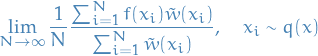
![\begin{equation*}
\begin{split}
\lim_{N \to \infty} \frac{1}{N} \frac{\sum_{i=1}^{N} f(x_i) \tilde{w}(x_i)}{\sum_{i=1}^{N} \tilde{w}(x_i)} &= \lim_{N \to \infty} \frac{1}{N} \sum_{i=1}^{N} f(x_i) \tilde{w}(x_i) \frac{Z_q}{Z_p} \\
&= \lim_{N \to \infty} \frac{1}{N} \sum_{i=1}^{N} f(x_i) \frac{\tilde{p}(x_i)}{Z_p} \frac{Z_q}{\tilde{q}(x_i)} \\
&= \lim_{N \to \infty} \frac{1}{N} \sum_{i=1}^{N} f(x_i) \frac{p(x_i)}{q(x_i)} \\
&= \mathbb{E}_q[f(x) w(x)] \\
&= \mathbb{E}_p[f(x)]
\end{split}
\end{equation*}](../../assets/latex/markov_chain_monte_carlo_f36c095dc18315473a72b11c739daffb95599f23.png)
with  . That is, as
  , taking the unnormalized weigth
  we arrive at the same result as if we used the proper weights
  .
.
Issues
Large number of dimensions
In a large number of dimensions, one will often have the problem that a small number of large weights  will dominate the the sampling process. In the case where large values of
  lie in low-probability regions this becomes a huge issue.
Rejection Sampling
- Have which is too complex to sample from
- We have a simpler density which we can evalute (up to a factor
 ) and raw samples from
 Assume that we know the value of a constant
 s.t.
s.t.
- For
 :
:
- Generate

- Generate
- Accept
 if
if  , reject
  if
if 
- Generate
Then
We're simply sampling from a distibution we can compute, and then computing the ratio of samples under  which also fell under . Since we then know the "area" under we know that the area under is simply the ratio of points accepted.
This is basically a more general approach to the [BROKEN LINK: No match for fuzzy expression: *Box%20method%20Sampling], where we instead of having some distribution to sample from, we simply use a n-dimensional box (or rather, we let be a multi-dimensional  ).
).
Issues
Large number of dimensions
In large number of dimensions it's very likley that the requirement
forces to be so huge that acceptances become very rare.
Even finding in a high-dimensional space might be incredibly difficult.
Markov Chain Monte Carlo (MCMC)
Markov chains
A Markov chain is said to be reversible if there is a probability distribution  over its states such that

for all times n and all states  and
and  . This condition is known as the detailed balance condition (some books call it the local balance equation).
Methods
Metropolis-Hastings
The family of Metropolis-Hastings MCMC methods all involve designing a Markov process using two sub-steps:
- Propose. Use some proposal distribution
 to propose the next state
  given the current state .
 - Acceptance-rejection. Use some acceptance distribution
 and accept / reject depending on this conditional distribution.
The transition probability is then

Inserting into the detailed balance equation for a MC we have
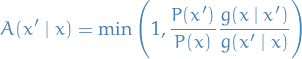
This is satisfied by (for example) the Metropolis choice:
The Metropolis-Hastings algorithm in its full glory is then:
- Initialize
- Pick initial state

- Set

- Pick initial state
- Iterate
- Generate: randomly generate a candidate state according to
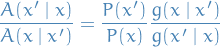
- Compute: compute acceptance probability
- Accept or Reject:
- Generate a uniform random number
![$u \in [0, 1]$](../../assets/latex/markov_chain_monte_carlo_78efdcf7fcc040ee4d3befbeb8a234cbf06df8d6.png)
- If
 , accept new state and set
- If
 , reject new state and set
- Generate a uniform random number
- Increment: set

- Generate: randomly generate a candidate state
The empirical distribution of the states  will approach
  .
.
When using MCMC methods for inference, it's important to remember that is usually the log-likelihood of the data.
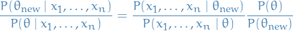
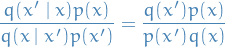
This can also be seen by considering the posterior distribution of the parameters given the data, and considering the ratio between two different parameters, say  and
and  . Then
Letting the prior-distribution on  be the proposal distribution
  in Metropolis-Hastings algorithm, we see that in this case we're simply taking steps towards the parameter which maximizes the log-likelihood under some prior.
Further, one could make the ratio  by using a uniform distribution (if we know that
 ![$\theta \in [a, b]$](../../assets/latex/markov_chain_monte_carlo_020b4191ce288e0fce00e0ee2e41e1b20e50026a.png) for some
for some  .
.
The choice of  is often referred to as a (transition) kernel when talking about different Metropolis-Hastings methods.
Gibbs
Gibbs sampling or a Gibbs sampler is a special case of a Metropolis-Hastings algorithm. The point of a Gibbs sampler is that given a multivariate distribution it is simpler to sample from a conditional distribution than to marginalize by integrating over a joint distribution.
Suppose we want to sample  from a join distribution
  . Denote k-th sample by
  . We proceed as follows:
- Initial value:

- Sample
 . For
. For  :
:
- Sample
 .
If sampling from this conditional distribution is not tractable, then see Step 2 in the Metropolis-Hastings algorithm for how to sample.
.
If sampling from this conditional distribution is not tractable, then see Step 2 in the Metropolis-Hastings algorithm for how to sample.
- Sample
- Repeat above step until we have the number of samples we want.
Proof of convergence
Suppose we want to estimate the for a state  .
.
Let
 denote the values which
  can take on, i.e.
  is all the possible states, keeping
  constant.
 denote some mass density over the indices
  (with non-zero mass everwhere)
Assuming  , the Gibbs procedure gives us
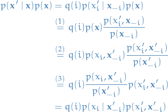
where in
 we used
 we used
 we used the fact that
Therefore we have

which implies the detailed balance equation is satisfied, hence is the stationary distribution of the resulting Markov Chain.
Further, to ensure that this stationary distribution actually exists, observe that we can reach any state  from the state
  in some number of steps, and that there are no "isolated" states, hence the chain constructed by the Gibbs transition creates an aperiodic and irreducible Markov Chain, which is guaranteed to converge to its stationary distribution .
In our definition of Gibbs sampling, we sample from the different dimensions sequentially, but here we have not assumed how sample the different dimensions, instead giving it some arbitrary distribution . Hence Gibbs sampling also works when not performing the sampling sequentially, but the sequential version is standard approach and usually what people refer to when talking about Gibbs sampling.
The notation  instead of is often when talking about Markov Chains. In this case we're mainly interested in sampling from a distribution , therefore we instead let denote the stationary distribution of the chain.
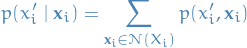
In a Markov Random Field (MRF) we only need to marginalize over the immediate neighbours, so the conditional distribution can be written
Convergence bound
If  is the transition matrix of the Gibbs chain, then the convergence rate of the periodic Gibbs sampler for the stationary distribution of an MRF is bounded by
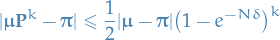
where
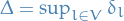

 is the arbitrary initial distribution
 is the distance in variation
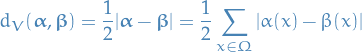
for distributions
 and
and  on a finite state space
Slice sampling
- Great introduction to it mackay2003information
- Alternatively, also from MacKay, see this lecture on the subject: https://www.youtube.com/watch?v=Qr6tg9oLGTA&t=4124s. I found this quite nice!
- Originally from neal00_slice_sampl
TODO Elliptical Slice sampling
Particle MCMC (PMCMC)
References:
TODO Sequential Monte-Carlo (SMC)
TODO Particle Gibbs (PG)
TODO Particle Gibbs with Backward Sampling (PGBS)
TODO Particle Gibbs with Ancestor Sampling (PGAS)
TODO Embedded MCMC (EMCMC)
Specific case: Hidden Markov-Models (HMMs)
Follows shestopaloff16_sampl_laten_states_high_dimen.
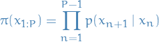
The following assumes a state-space model where
 is the initial latent state
 is the transition probability
 is the emission/observation probability
- denotes the number of time-steps in the SSM
- Current sequence is
- Update to as follows:
For each time
, generate a set of  "pool states", denoted by
![\begin{equation*}
\mathcal{P}_i := \left\{ x_i^{[1]}, \dots, x_i^{[L]} \right\}
\end{equation*}](../../assets/latex/markov_chain_monte_carlo_22b5f6f6c8ecff560e19be25df48d2d7004cb94b.png)
- Pool states are sampled independentlyo across different times
- Pool states are sampled independentlyo across different times
Choose
 uniformly at random and let
![\begin{equation*}
x_i^{[l_i]} := x_i
\end{equation*}](../../assets/latex/markov_chain_monte_carlo_25ec5a4e8639ab90e75a5c542249bc63abcb17e6.png)
- Sample remaining
 pool states
 ![$x_i^{[1]}, \dots, x_i^{[l_i - 1]}, x_i^{[k_i + 1]}, \dots, x_n^{[L]}$](../../assets/latex/markov_chain_monte_carlo_c563f8ef15b5fc82098f9f716a89100d65e6fc98.png) using Markov chain that leaves the pool density
using Markov chain that leaves the pool density  invariant:
Let
 be the transition prob of this Markov chain, with
  the transition for this chain reversed, i.e.
s.t.

for all
and .
- For
 :
:
- Generate
![$x_i^{[k]}$](../../assets/latex/markov_chain_monte_carlo_f7b0fcc5d69771abb1a576b62a8cb5edaa97463e.png) by sampling according to the reverse transition kernel
by sampling according to the reverse transition kernel ![$\tilde{R}_i\big(x_i^{[k]} \mid x_i^{[k + 1]}\big)$](../../assets/latex/markov_chain_monte_carlo_6824f1643142a2ad401765da90a3760e63292eca.png)
- Generate
- For
 :
:
- Generate by sampling according to the forward transition kernel
![$R_i\big(x_i^{[k + 1]} \mid x_i^{[k]}\big)$](../../assets/latex/markov_chain_monte_carlo_39cc2b3f7c590b9a010b043059f7a058556f5df6.png)
- Generate
- Generate new sequence using stochastic backwards pass:
- For each time , we then compute the forward probabilities
 , with taking values in
  :
:
if
 :
:
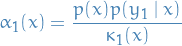
else:
![\begin{equation*}
\alpha_i(x) = \frac{p(y_i \mid x)}{\kappa_i(x)} \sum_{l=1}^{L} p\big(x \mid x_{i - 1}^{[l]} \big) \alpha_{i - 1} \big( x_{i - 1}^{[l]} \big)
\end{equation*}](../../assets/latex/markov_chain_monte_carlo_3892342e93dfccd3752b7d004af82aadb4f60602.png)
- Sample new state sequence using a "stochastic backwards pass" (?):
- Sample
 from
from  (pool states at time
  ) with probabilities prop. to
- For
 :
:
- Sample
 from
from  (pool states at time
  ) with probabilities prob. to
- Sample
- Sample
- For each time
Alternatively, we can replace step 4 above by instead computing the backward probabilities:
- For
 , compute backward probabilities
  with
with  :
:
if
 :
:

else:
![\begin{equation*}
\beta_i(x) := \frac{1}{\kappa_i(x)} \sum_{l=1}^{L} p \big( y_{i + 1} \mid x_{i + 1}^{[l]} \big) p \big( x_{i + 1}^{[l]} \mid x \big) \beta_{i + 1} \big( x_{i + 1}^{[l]} \big)
\end{equation*}](../../assets/latex/markov_chain_monte_carlo_80deb4ed80c383da0c4ca55b94351b820579b0ee.png)
- Sample new state sequence using a stochastic forward pass:
- Sample
 from with prob. prop. to
- For
 :
:
- Sample
 from with prob. prop. to
- Sample
- Sample
TODO Unification of PMCMC and EMCMC andrieu2010particle
Notation
 is an
is an  latent Markov process satisfying
 is a sequence of
  observations which are conditionally independent given and satisfy

or, with a slighy abuse of notation,

 denotes the parameters of the model
Particle Independent Metropolis-Hastings (PIMH)
- Independent Metropolis-Hastings (IMH) refers to the fact that the proposal distribution is independent of the current state
- Proof idea:
- Check that
 when
when 
Deduce that acceptance ratio of an IMH update with target
 and proposal density
  takes the form

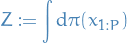
where
 denotes the estimate of the normalization constant for the proposition
- Check that
- Proof
- If we assume (1), then we can quickly see that
- Construct a kernel which leaves the extended target distribution invariant, which is defined in such a way that we also leave the actual target density invariant
and the particle estimate
Note that
TODO Particle marginal Metropolis-Hastings (PMMH)
- Extended target distribution
Proposal:
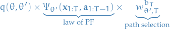
where
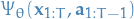 is the law induced by bootstrap/resampling PF:
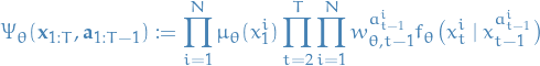
where
 is the prior for
 is the probability of the i-th particle taking on the value
  at time-step
  given that it's parent (indexed by
  ) has taken on the value
 is the probability of having chosen as the parent in for the i-th particle at time-step
Resulting MH acceptance step is
where
![\begin{equation*}
\hat{p}_{\theta}(y_{1:T}) := \prod_{t = 1}^{T} \bigg[ \frac{1}{N} \sum_{i=1}^{N} g_{\theta}\big(y_t \mid x_t^i\big) \bigg]
\end{equation*}](../../assets/latex/markov_chain_monte_carlo_7685556f1257bb37553364c9b06cca486707a069.png)
is an unbiased estimate of

The fact that it's correct can be shown by dividing the extended target by the probabililty of the auxillary variables:
since

and

PMCMC methods
- Notation
 denotes the number of particles
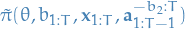
 represents the latent-state trajectory with "ancestor path"
  :
:
and thus
 is the indices of the reference path.
Particles are denoted by bold-face:
Ancestor particles
and
Extended target distribution on
 :
:

 denotes the parameter domain
 is the domain of the hidden states in the state-space model for each of the
  particles
 represents all possible ancestor particles we can "possible generate" (you know what I mean…) since
  for any choice of
  , i.e. the first node (the root) of a path does not have an ancestor.
- In our case of considering SSMs, we have

Conditional particle filter (CPF):

with
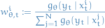
represents the normalized weight associated with the i-th particle at time
- Extended target distribution
To prove correctness we take the following approach:
- Find kernel which leaves the extended target distribution
 invariant
 - Show that the PGAS kernel on the original space is a collapsed version of this extended kernel
- Showing that a Gibbs kernel is a collapsed Gibbs can be done by considering a kernel on the extended space where some of the variables on the extended space is considered as auxillary variables
- For we're really just interested in the path chosen
 , and everything else is redundant information.
 - I.e.
- Note that
 is basically the product of the following distributions:
- From
 we pick the trajectory with indices
 - We consider this jointly with the probability of generating all these other trajectories
- Inputs:
- Parameters
- Candidate path
- Parameters
- Note that ancestor indices
 alone does not define a path! These define a path through already sampled set of particles . Hence we need both the particles and the ancestor indices to define a path
- From
- Find kernel which leaves the extended target distribution
- Proof of correctness
Finding a starting point
Burn-In
- Throw away some iterations at the beginning of an MCMC run
Issues
Dependent samples
The samples of a Markov Chain are in general dependent, since we're conditioning on the current state when sampling the proposal state.
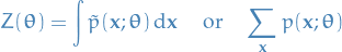
Partition function estimation
Notation
 is a unnormalized probability distribution
Probability distribution
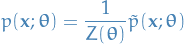
with
Overview
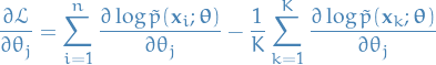
Log-likelihood is given by
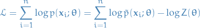
Gradient of  is then
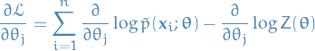
These two terms are often referred to as:
- postive phase
- negative phase
The 2nd term in the summation can be written:
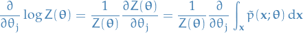
Interchanging integration and gradient, which we can do under under suitable conditions:
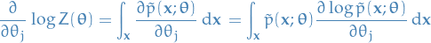
Hence,
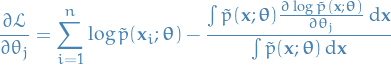
Since the  is constant, we observe that the second term in the above expression can be written
![\begin{equation*}
\begin{split}
\frac{\int \tilde{p}(\mathbf{x}; \boldsymbol{\theta}) \frac{\partial \log \tilde{p}(\mathbf{x} ; \boldsymbol{\theta})}{\partial \theta_j} \dd{\mathbf{x}}}{\int \tilde{p}(\mathbf{x}; \boldsymbol{\theta}) \dd{\mathbf{x}}}
&= \int \frac{\tilde{p}(\mathbf{x}; \boldsymbol{\theta})}{Z(\boldsymbol{\theta})} \frac{\partial \log \tilde{p}(\mathbf{x} ; \boldsymbol{\theta})}{\partial \theta_j} \dd{\mathbf{x}} \\
&= \mathbb{E}_p \big[ \log \tilde{p}(\mathbf{x}; \boldsymbol{\theta}) \big]
\end{split}
\end{equation*}](../../assets/latex/markov_chain_monte_carlo_5cd67c300a07c54f560cb5dd0d9d6581585caab3.png)
That is,
![\begin{equation*}
\frac{\partial \log Z(\boldsymbol{\theta})}{\partial \theta_j} = \mathbb{E}_p \big[ \log \tilde{p}(\mathbf{x}; \boldsymbol{\theta}) \big]
\end{equation*}](../../assets/latex/markov_chain_monte_carlo_01f06081fbcba2912eed95a6d7b5032e28f2be32.png)
And, employing MCMC algorithms, we can estimate this expectation as:
![\begin{equation*}
\mathbb{E} \big[ \log \tilde{p}(\mathbf{x}; \boldsymbol{\theta}) \big] \approx \frac{1}{K} \sum_{k=1}^{K} \log \tilde{p}(\mathbf{x}_k; \boldsymbol{\theta}), \quad \mathbf{x}_k \sim p(\ \cdot \ ; \boldsymbol{\theta})
\end{equation*}](../../assets/latex/markov_chain_monte_carlo_f1500d4a219c421aa6034fbb04d25cc410383776.png)
i.e.  are
are  MCMC samples from the unnormalized
  .
.
Finally, giving use a more tractable gradient estimate of :
The exact same argument holds for discrete random variables too, simply exchanging the integrand for a summation.
Problems
- Using standard MCMC methods, we would have to perform a burnin before sampling those samples in the negative phase. This can be very expensive.
- k-step Contrastive Divergence (CD-k): instead of initializing the chain from random samples, initialize from samples from the dataset.
Simulated Annealing (SA)
Simulated annealing is a method of moving from a tractable distribution to a distribution of interest via a sequence of intermediate distributions, used as an inexact method of handling isolated or spurrious modes in Markov chain samplers. Isolated modes is a problem for MCMC methods since we're making small changes between each step, hence moving from one isolated mode to another is "difficult".
It employes a sequence of distributions, with probability densities given by  to
to  , in which each
  differes only slightly from
  . The distribution
  is the one of interest. The distribution
  is designed so that the Markov chain used to sample from it allows movement between all regions of the state space.
A traditional scheme is to set

or the geometric average:
An annealing run is started from some initial state, from which we first simulate a Markov chain designed to converge to . Next we simulate some number of iterations of a Markov chain designed to converge to  , starting from the final state of the simulation for . Continue in this fashion, using the final state of the simulation for as the initial state of the simulation for
  , until we finally simulate the chain designed to converge to .
Unfortunately, there is no reason to think that annealing will give the precisely correct result, in which each mode of is found with exactly the right probability.
This is of little consequence in an optimization context, where the final distribution is degenerate (at the maximum), but it is a serious flaw for the many applications in statistics and statistical physics that require a sample from a non-degenerate distribution. neal98_anneal_impor_sampl
TODO Example: SA applied to RBMs
Annealed Importance Sampling (AIS)
- Combination of importance sampling and simulated annealing, where perform importance sampling on each of the distributions which converge to the target distribution
Annealed Importance Sampling (AIS)
Notation
 is a set of Gibbs distributions defined:
 , which we call the extended state space
- The use of square brackets, e.g.
![$\mathcal{P}[\cdot]$](../../assets/latex/markov_chain_monte_carlo_c4e5a48f9699437b729c73278438eb76253c993b.png) , denotes a distribution over
, denotes a distribution over 
We define
![\begin{equation*}
\mathcal{W}[\mathbf{x}] = - \ln \frac{\mathcal{P}[\mathbf{y}, x_N \mid x_0] p_0^*(x_0)}{\tilde{\mathcal{P}}[\mathbf{y}, x_0 \mid x_N] p_N^*(x_N)}
\end{equation*}](../../assets/latex/markov_chain_monte_carlo_fa2f8e27a0e5efdb3d4c0930b3caf609751e702e.png)
 (forward distribution) creates samples from
  given a sample from :
![\begin{equation*}
\mathcal{P}[\mathbf{x}] = P[\mathbf{y}, x_N \mid x_0] p_0(x_0)
\end{equation*}](../../assets/latex/markov_chain_monte_carlo_05d4f6198ebf69c33242bd8fa760ed53febd99ad.png)
 (reverse distribution) creates samples from given a sample
  from :
![\begin{equation*}
\tilde{\mathcal{P}}[\mathbf{x}] = \tilde{\mathcal{P}}[\mathbf{y}, x_0 \mid x_N] p_N(x_N)
\end{equation*}](../../assets/latex/markov_chain_monte_carlo_e6d67b940dbac5ddb322a2c9ee9b46089f01fda0.png)
Derivation
Assume that a set of Gibbs distributions  to construct a pair of distributions and on with
![\begin{equation*}
\begin{split}
\mathcal{P}[\mathbf{x}] &= P[\mathbf{y}, x_N \mid x_0] p_0(x_0) \\
\tilde{\mathcal{P}}[\mathbf{x}] &= \tilde{\mathcal{P}}[\mathbf{y}, x_0 \mid x_N] p_N(x_N)
\end{split}
\end{equation*}](../../assets/latex/markov_chain_monte_carlo_c61250e3341a007936028ba7810028989f0ef286.png)
- (forward distribution) creates samples from given a sample from
- (reverse distribution) creates samples from given a sample from
Then
![\begin{equation*}
\frac{\tilde{\mathcal{P}}[\mathbf{x}]}{\mathcal{P}[\mathbf{x}]} = \frac{Z_0 \tilde{\mathcal{P}}[\mathbf{y}, x_0 \mid x_N] p_N^*(x_N)}{Z_N \mathcal{P}[\mathbf{y}, x_N \mid x_0] p_0^*(x_0)} = \frac{Z_0}{Z_N} e^{-\mathcal{W}[\mathbf{x}]}
\end{equation*}](../../assets/latex/markov_chain_monte_carlo_ec33eee1887e132b874fa6a0d54fca64f77ef4b1.png)
where ![$\mathcal{W}[\mathbf{x}] = - \ln \frac{\mathcal{P}[\mathbf{y}, x_N \mid x_0] p_0^*(x_0)}{\tilde{\mathcal{P}}[\mathbf{y}, x_0 \mid x_N] p_N^*(x_N)}$](../../assets/latex/markov_chain_monte_carlo_cb3a70e8fc0ee2e23d74359c0d089e9a84bd5509.png) .
Then, for a function
.
Then, for a function  , we have
![\begin{equation*}
\tilde{\mathcal{P}}[\mathbf{x}] f(\mathbf{x}) = \mathcal{P}[\mathbf{x}] \frac{\tilde{\mathcal{P}}[\mathbf{x}]}{\mathcal{P}[\mathbf{x}]} f(\mathbf{x}) = \frac{Z_0}{Z_N} \mathcal{P}[\mathbf{x}] e^{- \mathcal{W}[\mathbf{x}]} f(\mathbf{x})
\end{equation*}](../../assets/latex/markov_chain_monte_carlo_9c409b8e0553d891da3f98215849ab2a93e172dd.png)
thus the expectation of
Then, letting  , i.e. constant function, we get
(Generalized) Annealed Importance Sampling (AIS) a method of estimating the partition function using the following relation:
where  is the partition function of the known "proxy" distribution .
The "standard" AIS method is obtained by a specific choice of .
Bennett's Acceptance Ratio (BAR) method
Bibliography
Bibliography
- [mackay2003information] MacKay, Kay & Cambridge University Press, Information Theory, Inference and Learning Algorithms, Cambridge University Press (2003).
- [neal00_slice_sampl] Neal, Slice Sampling, CoRR, (2000). link.
- [del2004feynman] @incollectiondel2004feynman, title=Feynman-kac formulae, author=Del Moral, Pierre, keywords = particle methods,mcmc, booktitle=Feynman-Kac Formulae, pages=47-93, year=2004, publisher=Springer, file=/home/tor/Dropbox/books/machine_learning/delmoral2004.pdf:PDF
- [chopin2020introduction] Chopin & Papaspiliopoulos, An introduction to sequential Monte Carlo,.
- [finke2015extended] @phdthesisfinke2015extended, title=On extended state-space constructions for Monte Carlo methods, author=Finke, Axel
- [shestopaloff16_sampl_laten_states_high_dimen] Shestopaloff & Neal, Sampling Latent States for High-Dimensional Non-Linear State Space Models With the Embedded Hmm Method, CoRR, (2016). link.
- [andrieu2010particle] Andrieu, Doucet & Holenstein, Particle markov chain monte carlo methods, Journal of the Royal Statistical Society: Series B (Statistical Methodology), 72(3), 269-342 (2010).
- [neal98_anneal_impor_sampl] Neal, Annealed Importance Sampling, CoRR, (1998). link.