Recursive Bayesian Filtering
Table of Contents
Notation
Kalman Filter
Assumed model
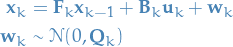
We assume the state to be random variable  as follows:
 1
1
and the measurements or observations to be a random variable  :
:
 2
2
I.e. both state and measurement are assumed
to be normally distributed with covariance-matrices  and
and  ,
respectively.
,
respectively.
Deduction
Notation
- state
 predicted state
 covariance matrix for the predicted state
 control-matrix, e.g. mapping external forces to how it affects the state
 control-vector, e.g. external force
- covariance matrix describing external uncertainty from the environment
 maps the predicted state to the measurement-space, i.e. "predict" measurement from state
- real measurement
- uncertainty in real measurements
Algorithm
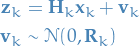
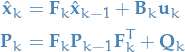
We start out by writing the predicted state  as a function of the previous
  predicted state:
 3
3
Where is due to the following identify:
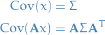 4
4
I.e. mapping the covariance at step  to the covariance of the state at step
  .
.
The next step is then to incorporate "external forces", where we use:
- - control vector which defines how
- - the matrix
I like to view  as a simple function mapping the control-vector to the state-space,
or rather, a function which maps the external "force" to how this "force" affects the state.
as a simple function mapping the control-vector to the state-space,
or rather, a function which maps the external "force" to how this "force" affects the state.
This, together with the uncertainty of the external "forces" / influences:
 5
5
Now, what if we can see the real measurement for step , , before proceeding?
Well, we would like to update our model! To do this, we need to relate the predicted state
to the real state . We thus write the predicted measurement as:
 6
6
Now, we can then write the real measurement as follows:
 7
7
And we of course want the following to be true:
 8
8
Therefore we can map the predicted state to the measurement-space by using the matrix .
Thus we have a model for making the predictions, now we need to figure out how to update our model!
For this we first map our "internal" state to the measurement-space. In this case, our measurements only consists of the position  .
.
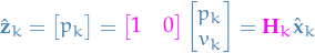
Thus, the predicted measurements follow  and the real measurements follow
  , where is the "real" internal state.
To compute our updated state, we can then take the joint distribution of the predicted and real measurements, incorporating information from both our estimate and the current measurement.
Due to the joint-probability of two Gaussian rvs. also being Guassian, with mean  and covariance
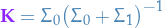
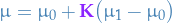
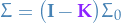
In the context of Kalman filters we call  the Kalman gain.
By letting  and
and  , we get the update-equations:


where  is without the in front.
Summary
Predict!
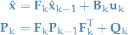 9
9
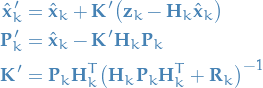
Update!
Since our predictive model is Gaussian, and we assume a Gaussian distribution for our measurements,
we simply update our model parameters  by taking the joint-distribution
of these two Gaussian rvs., which again gives us a Guassian distribution with the new updated paramters:
by taking the joint-distribution
of these two Gaussian rvs., which again gives us a Guassian distribution with the new updated paramters:
 10
10
Prediction
11
Update
Since our predictive model is Gaussian, and we assume a Gaussian distribution for our measurements, we simply update our model parameters by taking the joint-distribution of these two Gaussian rvs., which again gives us a Guassian distribution with the new updated parameters:
12
Particle Filtering
Notation
 denotes the k-th sampled step of the i-th "particle" / sample-sequence
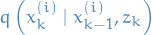 is the "importance distribution" which we can sample from
Overview
- Can represent arbitrary distributions
- But this is an approximate method, unlike method such as Kalman Filter which are (asymptotically) exact and "optimal"
- Name comes from the fact that we're keeping track of multiple "particles"
- "Particle" is just a single "chain" of samples
- Main building-block is Importance Sampling (IS)
- "Extended" to sequences, which we call Sequential Importance Sampling
Sequential Importance Sampling (SIS)
Sequential Importance Sampling (SIS) extends Importance Sampling (IS) by updating the sample-weights  sequentially.
The particle and weight updates, respectively, are defined by
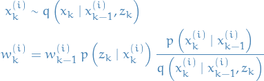
IMPORTANT: normalize the weights after each weight-update, such that we can use the weights to approximate the expectations.
![\begin{equation*}
\mathbb{E}[f(x_k)] = \frac{1}{N} \sum_{i=1}^{N} w_k^{(i)} f \left( x_k^{(i)} \right)
\end{equation*}](../../assets/latex/recursive_bayesian_filtering_c56d9b6133c36c0c4a8949b87b81bb83084a0415.png)
Degeneracy phenomenon
- Usually after a few iterations of SIS most particles have neglible weights
- => large computation efforts for updating particles with very small contributions: highly inefficient
One can "measure" degeneracy using the "effective sample size":
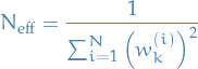
- Uniform:

- Severe degeneracy:

- Uniform:
- To deal with degeneracy we introduce resampling
- When degeneracy is above a threshold, eliminate particles with low importance weights
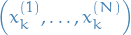
Sample
 new samples / "particles"
  by
by
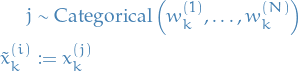
i.e. we're generating new particles by drawing from the current particles, each with probability equal to the corresponding weight.
- If we eliminiated the particles with low importance weights, the corresponding weights should of course not be included.
New samples and weights are

i.e. new weights are uniform.
A good threshold is a "measure" of degeneracy using the "effective sample size":
- Uniform:
- Severe degeneracy:
Practical considerations
Implementing the categorical sampling method used in resampling can efficiently be performed by
- Normalize weights
- Calculate an array of the cumulative sum of the weights
- Partitions the range
![$[0, 1]$](../../assets/latex/recursive_bayesian_filtering_68c8fa38d960e53d4308cbf1e65d04c66a554817.png) into intervals
into intervals - If
 , then the interval
  falls into is the corresponding
- Partitions the range
- Randomly generate uniform numbers
 and determine the corresponding samples
Generic Particle Filtering
Combining SIS and resampling, we get generic Particle Filtering.
At each "step" , we "obtain new states" / "update the particles" through:
- Produce tuple of samples
 using SIS
 - Compute

- If
 : resample!
- If