Linear Regression
Table of Contents
Multivariable linear regression
Assumptions
- Linearity
- Homoscedasticity
- A sequence of rvs. is homoscedastic if all rvs. in the sequence have the same finite variance
- The complementary notion sis called heteroscedasticity
- Multivariate normal
- Independence of errors
- Lack of multicolinearity
- For our estimator to be a Best Linear Unbiased Estimator (BLUE) we require that the variables are independent
Dummy variable trap
Let's say we have a categorical variable in our data set, which can
take on two values, e.g. raining or not raining
We can then either represent this as one binary variable,  or two binary variables,
  and
and  .
.
If we do one variable, we have the model:
 1
1
If we have two variables, we have the model:
 2
2
Now, do you see something wrong with the second option?
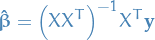
To obtain our estimated parameters  (when using Ordinary Least Squares (OLS))
we compute the following:
(when using Ordinary Least Squares (OLS))
we compute the following:
 3
3
where  is the
  data matrix and
  is the
  label-vector.
The issue lies in the  . To be able to compute a the inverse of
a matrix we require it to be invertible / non-singular. This is equivalent
of saying it needs to have full rank, i.e. all columns must be linearly independent
(The same holds for rows). In the case where
. To be able to compute a the inverse of
a matrix we require it to be invertible / non-singular. This is equivalent
of saying it needs to have full rank, i.e. all columns must be linearly independent
(The same holds for rows). In the case where  , this is not the case!
The covariance between and will be 1!
, this is not the case!
The covariance between and will be 1!
Therefore, you always go with the first solution. This also is the case for
categorical variables which can take on more than 2 values: you only include
a parameter  for
for  of these values the categorical variable
can take on.
of these values the categorical variable
can take on.
Intuitively, you can also sort of view it as the last value for the categorical
variable being included in the  .
.
Variable selection
This section is regarding choosing variables to include in your model, as you usually don't want to include all of them.
The three first methods (all different versions of "step-wise" regression) are apparently not a good idea:
Backward elimination
- Decide on some significance level, e.g.

- Fit full model using all variables
- Consider the variable with the largest P-value.
If
 :
:
- Go to step 4
- Otherwise: go to FIN
- Remove this variable.
- Fit full model without the removed variables. Go back to step 3
Forward elimination
- Decide on some significance level, e.g.
- Fit all simple regression models
 , and select the one with the lowest P-value
 - Keep this variable and fit all possible models with one extra predictor added to the one(s) you already have
- Consider the predictor with the lowest P-value.
If
 :
:
- Go to step 3, i.e. keep introductin predictors until we reach a insignificant one
- Otherwise: go to FIN
Since the last added predictor is of a too high P-value, we actually use the model fitted just before adding this last predictor, not the model we have when we go to FIN.
Bi-directional elimination (step-wise regression)
- Select a significance level to enter and to stay in the model,
e.g.:
SLENTER = 0.05andSLSTAY = 0.05 - Perform the next of Forward Selection (new variables must have: =P < SLENTER to enter)
- Perform ALL steps of Backward Elimination (old variables must have
P < SLSTAYto stay) - No new variables can enter and no old variables can exit => FIN
Recursive feature elimination
This one was not actually in the course-lectures, but is the only one provided as a
function by scikit-learn so I figured I'd include it. sklearn.featureselection.RFE.
- Decide on some number of features you want.
- Train estimator on the initial set of features and weights are assigned to each one of them
- Features whose absolute weights are the smallest, are pruned from the current set of features
- Procedure is recursively repeated on the pruned set until the desired number of features to select is eventually reached.
Geometric interpretation
Before you engage on this journey of viewing Multivariate Linear Regression in the light of geometry, you need to get the following into your head:
- Linear! Say it after me: lineeaar.
OKAY! So I'm smart now, we got dis.
SO! Let's consider the case of simple univariate (ONE SINGLE FREAKING VARIABLE), even excluding the bias / intercept, with the model:
 4
4
- is the input random variable
 is the dependent random variable
We then obtain our least squares estimate to be:
 5
5
 is a
is a  matrix (generally
  )
)- is a matrix
 is a
is a  matrix (generally
  )
)
Now, since we're only considering the univariate linear regression, we can instead use vector notation and end up with the following:
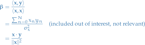 6
6
DO YOU SEE IT?!
just happens to be equal to the projection of our samples for the depedent variable onto the column space
of our samples for the feature / input variable. Interesting, or what?!
All-in-all, our least squares estimate is then the projection of our samples, , for the dependent rv. , onto the column-space
of our samples, , for the input rv. .
When we are making a prediction on some new input  , we're not
computing a projection!
, we're not
computing a projection!
This isn't hard to tell by looking at the equations, but I've found myself pondering about "how making a prediction is computing a projection" when we're not actually doing that.. #BrainFarts
Projections are for fitting and we're computing them for each feature / input variable with the corresponding observed label / dependent variable. These projections then give us the coefficient for the corresponding feature / input variable. Thus, when making a prediction we're computing a linear combination of the features / input variables where the coefficient for each of these are computed by what we described above.
TL;DR: Projections are for fitting, not predicting.
"But Tor, this is just univariate linear regression! We want to play with the big-boys doing multivariate linear regression!"
You see, my sweet summerchild, by making sure that our input variables are linearly independent, we can
simply provide each of the symbols above with a subscript  denoting the
  feature / input variable, and we're good!
For a more complete explanation of the multivariate case, checkout section 3.2 in The Elements Of Statistical Learning.
I tried…
We'll be viewing the least squares estimate as a projection onto the
column space of the data, . Why does this make any sense?
- Consider
 → instead of the other way around, i.e. given some
we want can define it
→ instead of the other way around, i.e. given some
we want can define it - Basically, the question we have here is "why does making the predicted
value for the projection onto the space spanned by the indep. variable
make the residuals smallest?"
- By def. the projection of some vector onto a subspace is defined to
such that the vector from its projected vector to is
perpendicular to the plane, i.e.
 is perpendicular
to subspace spanned by , i.e. minimal! (since perpendicular distance is the
smallest distance from the plane)
is perpendicular
to subspace spanned by , i.e. minimal! (since perpendicular distance is the
smallest distance from the plane) - Why is this relevant? Well, it tells us that if we have a set of orthogonal
vectors we can view our fit as a projection onto the column-space of all
 ,
i.e. the projection defines how much we move along each of the to get
our least estimate for some .
,
i.e. the projection defines how much we move along each of the to get
our least estimate for some . - EACH COMPONENT OF IS PROJECTED ONTO A SUBSPACE SPANNED BY THE INPUTS FOR THIS
SPECIFIC COMPONENENT!!!
- By def. the projection of some vector
from functools import wraps

import numpy as np
import matplotlib.pyplot as plt
import seaborn as sns


def ols_fit(X, y):
    # the code below is to standardize the inputs
    # X = X - X.mean()  # p x n
    # X = X / X.var()
    # need to account for intercept / bias
    beta_0 = np.ones(X.shape)
    X = np.vstack((beta_0, X))
    XX_inv = np.linalg.inv(np.dot(X, X.T))  # p x p
    beta = np.dot(np.dot(XX_inv, X), y.T)  # p x 1

    def predict(x):
        x = np.vstack((np.ones(x.shape), x))
        return np.dot(beta.T, x)  # p x n
    return predict

n = 10
x = np.arange(n).reshape(1, -1)
epsilon = np.random.normal(0, 1, n).reshape(1, -1)
y = np.arange(10, 10 + n).reshape(1, -1) + epsilon
fit = ols_fit(x, y)
y_fit = fit(x)
print(y_fit)

plt.scatter(x, y, label="$y$")
plt.scatter(x, y_fit, c="g", label="$\hat{y}$")
x_extra = (np.max(x) - np.min(x)) * 0.2
plt.xlim(np.min(x) - x_extra * 0.5, np.max(x) + x_extra)
y_extra = (np.max(y) - np.min(y)) * 0.2
plt.ylim(np.min(y) - y_extra, np.max(y) + y_extra)
plt.legend()
plt.title("Linear with white noise and fitted values")
plt.savefig(".linear_regression/1d_data.png")
return ".linear_regression/1d_data.png"
import numpy as np

n = 10
x = np.arange(n).reshape(1, -1)
epsilon = np.random.normal(0, 1, n).reshape(1, -1)
y = np.arange(10, 10 + n).reshape(1, -1) + epsilon

x = x - x.mean()
x /= x.var()
np.linalg.matrix_rank(x)
Estimating std. err. of parameter-estimates
So, we now have our parameter-estimates:
Now, the linear regression model is
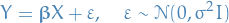
Thus, with our estimate for the parameters,
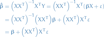
Here we're using to denote the true parameters.
which is a random variable following the distribution
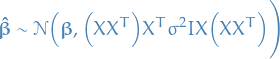
Thus we can compute the variance of each of the parameters, and therefore the standard error!
Least Squares Estimate
Bias-variance decomposition
Consider the mean squared error of an estimator  in estimating
![\begin{equation*}
\text{MSE}(\hat{\theta}) = E \Big[ (\hat{\theta} - \theta)^2 \Big]
\end{equation*}](../../assets/latex/linear_regression_633723fa83d74704152b51f58da6a821d6208c22.png) 7
7
The bias-variance decomposition would then be:
![\begin{equation*}
\begin{split}
\text{MSE}(\hat{\theta}) &= E \Big[ \big( \hat{\theta} - E(\hat{\theta}) + E(\hat{\theta}) - \theta \big)^2 \Big] \\
&= E \Big[ \big(\hat{\theta} - E(\hat{\theta}) \big) ^2 + \big(E(\hat{\theta}) - \theta \big)^2 \Big] \\
&= E \Big[ \big(\hat{\theta} - E(\hat{\theta}) \big) ^2 \Big] + E \Big[ \big(E(\hat{\theta}) - \theta \big)^2 \Big] \\
&= \text{Var}(\hat{\theta}) + \big( E[\hat{\theta}] - \theta \big)^2 \\
&= \text{Var}(\hat{\theta}) + E[\hat{\theta} - \theta]^2 \\
&= \text{Var}(\hat{\theta}) + \text{Bias}^2 (\hat{\theta})
\end{split}
\end{equation*}](../../assets/latex/linear_regression_36ba9a71395025052f60b09e51f3fbc6514d54fb.png) 8
8
Where ![$E \Big[ \big(E(\hat{\theta}) - \theta \big)^2 \Big] = \big( E(\hat{\theta}) - \theta) \big)^2$](../../assets/latex/linear_regression_ab9e84aac44f12908f2a8146ed00e865af671239.png) since both
since both  and are constant
Regularization methods
Ridge regression
Ridge regression shrinks the regression coefficients by imposing a penalty on their size.
Ridge regression minimizes a penalized residual sum of squares,
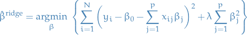
Here  is a complexity parameter that controls the amount of shrinkage; the larger the value of
  , the greater the amount of shrinkage.
An equivalent way to write the ridge problem is
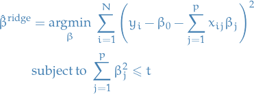
for some  .
.
There is a one-to-one correspondance between these two formalations, since the Lagrangian of this constrained optimization problem would only have an extra term of  , which would simply be a positive constant.
Using centered inputs, we drop and can write the problem in matrix form:

which have solutions

Ridge solutions are not equivariant under scaling of the inputs, and so one normally standardizest he inputs before solving.
The intercept has been left out of the penalty term! Penalization of the intercept would make the procedure depend on the origin chosen for , that is, adding a constant to each of the targets would not simply result in a shift of the predictions by the same amount  .
.
From ridge solution in matrix form, we see that the solution adds a positive constant to the diagonal of  before inversion. This makes the problem non-singular, even if is not!
This was the main motivation for ridge regression when it was first introduced.trevor09
Using Singular Value Decomposition of the centered input matrix  :
:

For "standard" least squares we have
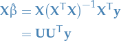
Observe that  , where
 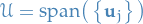 .
.
In comparison, the ridge solution is gives us
Note that since , we have

Observe that like linear regression, ridge regression computes the projection of onto the subspace spanned by  , but also shrinks these coordinates by the factors
  ! This is why you will sometimes see such methods under the name "shrinkage methods".
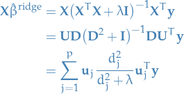
Variance
Since  is the sample covariance, we know that the eigenvectors of this,
  are the principal components of the variables in . Therefore, letting
  , we have
Hence, the small singular values  correspond to the directions in the column space of having small variance, and ridge regression shrinks these directions the most.
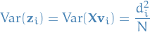
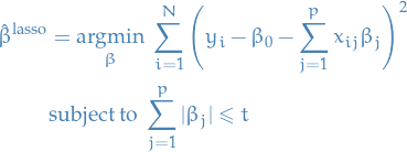
Lasso regression
Lasso regression is defined by the estimate
In the signal processing literature, the lasso is also known as basis pursuit.
We can write the lasso in the equivalent Lagrangian form:
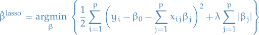
The absolute value here makes the optimization problem non-linear, and so there is no closed form expression as in the case of ridge regression.
Kernel methods
Different regression-models
Poission regression
Instead of assuming that  to follow

we assume

Bibliography
Bibliography
- [trevor09] Trevor Hastie, The elements of statistical learning : data mining, inference, and prediction, Springer (2009).