Factor-based models
Table of Contents
Principal Component Analysis (PCA)
Notation
 and
and  denotes the i-th eigenvector
 denotes the covariance-matrix
 is the eigenmatrix
Stuff
Principle Component Analysis (PCA) corresponds to the finding the
eigenvectors and eigenvalues of the (centered, i.e.  for each column
  )
covariance matrix of the data. We can do this since the covariance matrix
is the semi-positive definite matrix given by
)
covariance matrix of the data. We can do this since the covariance matrix
is the semi-positive definite matrix given by  .
.
If:
 is the
  data matrix
Think about it in this way:
- Eigenvectors form an orthogonal basis for the covariance matrix of the variables / features, i.e. we have a way of expressing the variances independently of each other.
- For each eigenvector / basis , the greater the corresponding
eigenvalue
 , the greater the explained variance.
 By projecting the data
onto this basis, simply by taking the matrix product
 , where
  is the matrix with columns corresponding to the eigenvectors
of the
is the matrix with columns corresponding to the eigenvectors
of the  covariance matrix
  , we have a new "view" of the
features where
, we have a new "view" of the
features where
![$x_i^T V = [x_i^T v_1, ..., x_i^T v_p], \quad \forall i \in \{1, ..., n\}$](../../assets/latex/factor_based_models_f1a4d100fb0862f84426d8f6340e7fb5f42ab705.png) i.e. we are now looking at
each data point transformed to a space where the basis vectors are linearly
independent, each explaining some of the variance of the features in the
data.
i.e. we are now looking at
each data point transformed to a space where the basis vectors are linearly
independent, each explaining some of the variance of the features in the
data.
Now we make another observation:
- Take the Singular Value Decomposition (SVD) of :
 X = U Σ VT
Then,
 1
1
Thus we in actually only need to compute the SVD of the data matrix
to be
able to compute the entire covariance matrix  !
!
What does the eigenvalue
actually tell us?
 =>
=> ![$CV = [\sigma_1^2 \mathbf{v}_1, ..., \sigma_p^2 \mathbf{v}_p], \quad \text{since } \lambda_i = \sigma_i^2$](../../assets/latex/factor_based_models_2d5fc0250fe02b6da83eb136f285648985dae722.png) where
where 
- Take the Singular Value Decomposition (SVD) of
PCA maximum variance formulation using Lagrange multipliers
Want to consider a projection of the data onto a subspace which maximizes the variance, i.e. explains the most variance.
- Let
 be the direction of this subspace, and we want to be a unit vector, i.e.
- Each data point
 is then projected onto the scalar
- The mean of the projected data is

Variance of projected data is:

Then to maximize the variance of the projected data  wrt. under the constraint .
We then introduce the Lagrange multiplier  and define the unconstrained maximization of

By taking the derivative wrt. and setting to zero, we observe that the solution satisfies:

i.e. must be an eigenvector of with eigenvalue .
We also observe that,

due to being an eigenvector of . We call the first principal component.
To get the rest of the principal components, we simply maximize the projected variance amongst all possible directions orthogonal to those already considered, i.e. constrain the next  such that
  .
.
TODO Figure out what the QR representation has to do with all of this
Whitening
Notation

![$\mathbf{V} = [\mathbf{v}_1 \ \dots \ \mathbf{v}_D]$](../../assets/latex/factor_based_models_aba2170ba2d7ed902b4a3e74f0b8254a685c708d.png) is matrix with the normalized eigenvectors, i.e. an orthonormal matrix
is matrix with the normalized eigenvectors, i.e. an orthonormal matrix is the whitened data
Stuff
- Can normalize the data to give zero-mean and unit-covariance (i.e. variables are decorrelated)
Consider the key eigenvalue problem in PCA in a matrix form;
![\begin{equation*}
\boldsymbol{\Sigma} \mathbf{V} = \mathbf{V} \mathbf{L}, \quad \mathbf{L} = \text{diag} \big( \lambda_1, \dots, \lambda_D \big), \quad \mathbf{V} = [\mathbf{v}_1 \ \dots \ \mathbf{v}_D] \ \text{(orthogonal)}
\end{equation*}](../../assets/latex/factor_based_models_0581c7d0811467f459458978e1bca61932eee91f.png)
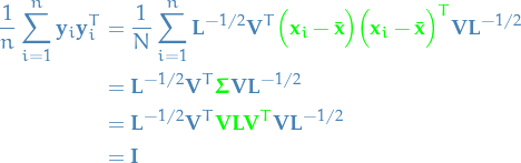
For each data point , we define a transformed value as:
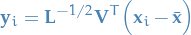
Then the set  has zero mean and its covariance is the identity:
Difference between PCA and OLS
set.seed(2)

x <- 1:100
epsilon <- rnorm(100, 0, 60)
y <- 20 + 3 * x + epsilon

plot(x, y)

yx.lm <- lm(y ~ x)  # linear model y ~ x
lines(x, predict(yx.lm), col="red")

xy.lm <- lm(x ~ y)
lines(predict(xy.lm), y, col="blue")

# normalize means and cbind together
xyNorm <- cbind(x = x - mean(x), y = y - mean(y))
plot(xyNorm)

# covariance
xyCov <- cov(xyNorm)
eigenValues <- eigen(xyCov)$values
eigenVectors <- eigen(xyCov)$vectors

plot(xyNorm, ylim=c(-200, 200), xlim=c(-200, 200))
lines(xyNorm[x], eigenVectors[2,1] / eigenVectors[1, 1] * xyNorm[x])
lines(xyNorm[x], eigenVectors[2,2] / eigenVectors[1, 2] * xyNorm[x])

# the largest eigenValue is the first one
# so that's our principal component.
# But the principal component is in normalized terms (mean = 0)
# and we want it back in real terms like our starting data
# so let's denormalize it

plot(x, y)
lines(x, (eigenVectors[2, 1] / eigenVectors[1, 1] * xyNorm[x]) + mean(y))

# what if we bring back our other two regressions?
lines(x, predict(yx.lm), col="red")
lines(predict(xy.lm), y, col="blue")
Factor Analysis (FA)
Overview
Factor analysis is a statistical method used to describe variability among observed, correlated variables in terms of a lower number of unobserved variables called factors.
It searches for joint variations in response to unobserved latent variables.
Notation
- set of
 observable random variables
  with means
 are common factors because they influence all observed random variables, or in vector notation
 denotes the
  matrix which represents our samples for the rvs.
  denotes the number of common factors ,
 is called the loading matrix
 is unobserved stochastic error term with zero mean and finite variance
Definition
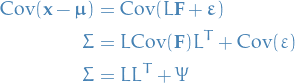
We suppose that the set of observable random variables with means , we have the following model:

or in matrix terms,

where if we have  observations:
  . (Notice that here is a matrix, NOT a vector, but in our model is vector. Matrix is for fitting, is the random variable we're modelling. Confusing notation, yeah I know.)
We impose the following conditions on :
- and
 are independent
 ![$\mathbb{E}[\mathbf{F}] = 0$](../../assets/latex/factor_based_models_96e0059ec063ff70cf9adcd9736ad9ba30cd64e6.png)
 (to make sure that the factors are uncorrelated, as we hypothesize)
Suppose  . Then note that from the conditions just imposed on , we have
In words
What we're saying here is that we believe the data can be described by some linear (lower-dimensional) subspace spanned by the common factors , and we attempt to find the best components for producing this fit. The matrix describes the coefficients for the observed rvs. when projecting these onto the common factors.
This is basically a form of linear regression, but instead of taking the observed rvs.  and directly finding a subspace to the data onto to predict some target variable, we instead make the observed "features"
  the target and hypothesize that there exists some common factors which produces the variance seen between the observed variables.
In a way, it's very similar to PCA, but see PCA vs. Factor analysis for more on that.
Exploratory factor analysis (ETA)
Same as FA, but does not make any prior assumptions about the relationships among the factors themselves, whereas FA assumes them to be independent.
PCA vs. Factor analysis
PCA does not account for inherit random error
In PCA, 1s are put in the diagonal meaning that all of the variance in the matrix is to be accouned for (including variance unique to each variable, variance common among variables, and error variance).
In EFA (Exploratory Factor Analysis), the communalities are put in the diagonal meaning that only the variance shared with other variables is accounted for (excluding variance unique to each variable and error variance). That would, therefore, by definition, inlcude only variance that is commong among the variables.
Summary
- PCA is simply a variable reduction technique; FA makes the assumption that an underlying causal model exists
- PCA results in principal components analysis that account for maximal amount of variance of observed variables; FA account for variance shared between observed variables in the data.
- PCA inserts ones on the diagonals of the correlation matrix; FA adjusts the diagonals of the correlation matrix with the unique factors.
- PCA minimizes the sum of squared perpendicular distance to the component axis; FA estimates factors which influence responses on observed variables.
- The component scores in PCA represent a linear combination of observed variables weighted by the eigenvectors; the observed variables in FA are linear combinations of the underlying unique factors.
Indendent Factor Analysis (ICA)
Overview
- Method for separating a multivariate signal into additive subcomponents
- Assumes subcomponents are non-Gaussian signals
Assumptions
- Different factors are independent of each other (in a probabilistic sense)
- Values in each factor have non-Gaussian distributions
Defining independence
We want to maximize the statistical independence between the factors. We may choose one of many ways to define a proxy for independence, with the two broadest ones:
- Minimization of mutual information
- Uses KL divergence and maximum entropy
- Maximization of non-Gaussianity
Definition
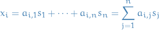
In a Linear Noiseless ICA we assume components of an observed random vector  are generated as a sum of (statistically) independent components
  , i.e.
for some  .
.
In matrix notation,

where the problem is to find the matrix  .
.
In a Lineary noisy ICA we follow the same model as for the noiseless ICA but with the added assumption of zero-mean and uncorrelated Gaussian noise

where  .
.
Comparison
- PCA maximizes 2nd moments, i.e. variance
- Finding basis vectors which "best" explain the variance of the data
- FA attempts to
- Generative
- Allows different variances across the different basis vectors
- ICA attempts to maximize 4th moments, i.e. [BROKEN LINK: No match for fuzzy expression: def:kurtosis]
- Finding basis vectors such that resulting vector is one of the independent components of the original data
- Can do this by maximizing kurtosis or minimizing mutual information
- Motivated by the idea that when you add things up, you get something normal, due to CLT
- Hopes that data is non-normal, such that non-normal components can be extracted from them
- In attempt to exploit non-normality, ICA tries to maximize the 4th moment of a linear combination of the inputs
- Compares to PCA which attempts to do the same, but for 2nd moments
- Finding basis vectors such that resulting vector is one of the independent components of the original data