Expectation propagation
Table of Contents
Notation
 denotes the Kullback-Leibler divergence, to be minimized wrt.
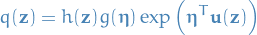
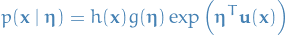
- is the approximate distribution, which is a member of the exponential family, i.e. can be written:
 is a fixed distribution
 denotes the data
 denotes the parameters / hidden variables
Exponential family
The exponential family of distributions over  , given parameters
  , is defined to be the set of distribtions of the form
where:
- may be discrete or continuous
 is just some function of
MLE
If we wanted to estimate in a density of the exponential family, we would simply take the derivative wrt of the likelihood of the distribution and set to zero:
![\begin{equation*}
\nabla g(\boldsymbol{\eta}) \int h(\mathbf{x}) \exp \Big[ \boldsymbol{\eta}^T \mathbf{u}(\mathbf{x}) \Big] \ d \mathbf{x} + g (\boldsymbol{\eta}) \int h(\mathbf{x}) \exp \Big( \boldsymbol{\eta}^T \mathbf{u}(\mathbf{x}) \Big) \ d \mathbf{x} = 0
\end{equation*}](../../assets/latex/expectation_propagation_972053bacb00408c653dac45e4b484d2ef130081.png)
Rearranging, we get
![\begin{equation*}
- \frac{1}{g(\boldsymbol{\eta})} \nabla g(\boldsymbol{\eta}) = g(\boldsymbol{\eta}) \int h(\mathbf{x}) \exp \Big( \boldsymbol{\eta}^T \mathbf{u}(\mathbf{x}) \Big) = \mathbb{E} \big[ \mathbf{u}(\mathbf{x}) \big]
\end{equation*}](../../assets/latex/expectation_propagation_0988d130774728543fdfcb4434c3760e5c30f240.png)
which is just
![\begin{equation*}
- \nabla \ln g(\boldsymbol{\eta}) = \mathbb{E} \big[ \mathbf{u}(\mathbf{x}) \big]
\end{equation*}](../../assets/latex/expectation_propagation_d0684a8d69080cdc07fccf176c53f15774df3188.png)
The covariance of can be expressed in terms of the second derivatives of  , and similarily for higher order moments.
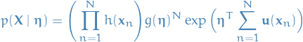
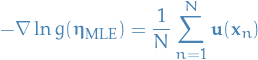
Thus, if we had set of i.i.d. data denoted by  , for which the likelihood function is given by
which is minimized wrt. when
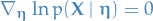
giving us the MLE estimator
i.e. the MLE estimator depends on the data only through  , hence is a sufficient statistic.
Minimizing KL-divergence between two exponential distributions
The KL divergence then becomes
![\begin{equation*}
\text{KL}(q || p) = - \ln g(\boldsymbol{\eta}) - \boldsymbol{\eta}^T \mathbb{E}_{p(\mathbf{z})} \big[ \mathbf{u}(\mathbf{z}) \big] + \text{const}
\end{equation*}](../../assets/latex/expectation_propagation_1766edade4cfe9ef8c3bc3dddde863854719b4ce.png)
where ,  and
and  define the approximation distribution
  .
.
We're not making any assumptions regarding the underlying distribution of  .
.
Which is minimized wrt. by
![\begin{equation*}
- \nabla \ln g(\boldsymbol{\eta}) = \mathbb{E}_{p(\mathbf{z})} \big[ \mathbf{u}(\mathbf{z}) \big]
\end{equation*}](../../assets/latex/expectation_propagation_4c7ab2596eed595fa2d300a7f7516bbccfd3520d.png)
From MLE estimator for exponential we then have
![\begin{equation*}
\mathbb{E}_{q(\mathbf{z})} \big[ \mathbf{u}(\mathbf{z}) \big] = \mathbb{E}_{p(\mathbf{z})} \big[ \mathbf{u}(\mathbf{z}) \big]
\end{equation*}](../../assets/latex/expectation_propagation_2eb09592c9e79caefd1bcbba1ce46f345bcffa0d.png)
hence, the optimum solution corresponds to matching the expected sufficient statistics!
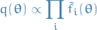
Expectation propagation
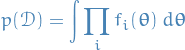
Joint probability of data and parameters given by
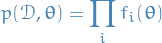
Want to evaluate
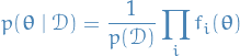
and
 for model comparison:
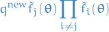
Expectation propagation is based on the approximation to the posterior distribution
 by
by 
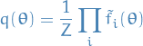
where
 is an approximation to the factor
  in the true posterior
- To be tractable, need to constrain the approximators
 => assume to be exponential
 Want to determine
by minimizing KL divergence between true and approx. posterior:
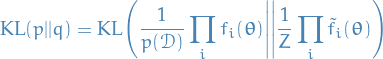
One approach of doing this would be to minimize KL divergence between the pairs and of factors.
It turns out that this no good; even though each of the factors are approximated individually, the product could still give a poor approximation.
(Also, if our assumptions are not true, i.e. true posterior is actually not of the exponential family, then clearly this approach would not be a good one.)
Expectation propagation optimizes each factor in turn, given the "context" of all remaining factors.
Suppose we wish to update our estimate for  , then we would like the following (assuming data was drawn from some exponential distribution):
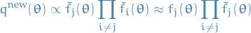
i.e. want to optimize for the j-th factor conditioned on our estimate for all the other factors. (Expectation maximization, anyone?)
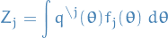
This problem we can pose as minimizing the following KL divergence
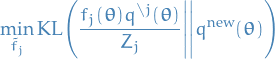
where:
new approximate distribution:
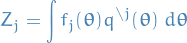
the unnormalized distribution:
normalization with
 replaced by
  :
:
Which we already know comes down to having:

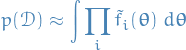
and we wish to approximate the posterior distribution by a distribution of the form

and the model evidence .
- Initialize all of the approximating factors
Initialize the posterior approximation by setting
- Until convergence:
- Choose a factor to improve
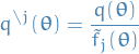
Remove
from posterior by division:

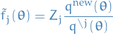
Let
 be such that
![\begin{equation*}
\mathbb{E}_{q^{\backslash j} f_j(\boldsymbol{\theta}) / Z_j}(\boldsymbol{\theta})}\big[ \mathbf{u}(\boldsymbol{\theta}) \big] = \mathbb{E}_{q^{\text{new}}(\boldsymbol{\theta})} \big[ \mathbf{u}(\boldsymbol{\theta}) \big]
\end{equation*}](../../assets/latex/expectation_propagation_5c53c177adea014bd11d13fb94f6c4b39e6b9470.png)
i.e. matching the sufficient statistics (moments) of
with those of  , including evaluating the normalization constant
Evaluate and store new factor
- Choose a factor
Evaluate the approximation to the model evidence:
Notes
- No guarantee that iterations will converge
- Fixed-points guaranteed to exist when the approximations are in the exponential family
- So at least then it converges, but to what? Dunno
- Can also have multiple fixed-points
- However, if iteratiors do converge; resulting solution will be a stationary point of a particular energy function (although each iteration is not guaranteed to actually decrease this energy function)
- Fixed-points guaranteed to exist when the approximations are in the exponential family
- Does not make sense to apply EP to mixtures as the approximation tries to capture all of the modes of the posterior distribution
Moment matching / Assumed density filtering (ADF): a special case of EP
- Initializes all to unity and performs a single pass through the approx. factors, updating each of them once
- Does not make use of batching
- Highly dependent on order of data points, as
 are only updated once