Expectation Maximization (EM)
Table of Contents
Summary
Expectation Maximization (EM) is an algorithm for obtaining the probability of some
hidden random variable  given some observations
  .
.
It is a two-step algorithm, which are repeated in order until convergence:
Expectation-step: Choose some probability distribution
 ,
,
 1
1
which gives us a (tight) lower-bound for
 for the curren estimate of
Maximization-step: optimize the
 2
2
Or rather, following the notation of Wikipedia:
Expectation step (E step): Calculate (or obtain an expression for) the expected value of the (complete) log likelihood function, with respect to the conditional distribution of
 given
given  under the current estimate
of the parameters
under the current estimate
of the parameters  :
:
![\begin{equation*}
Q(\boldsymbol\theta|\boldsymbol\theta^{(t)}) = \operatorname{E}_{\mathbf{Z}|\mathbf{X},\boldsymbol\theta^{(t)}}\left[ \log L (\boldsymbol\theta;\mathbf{X},\mathbf{Z}) \right]
\end{equation*}](../../assets/latex/expectation_maximization_6806dedd4d093a43a1b7351e6c826f2d45f05e62.png) 3
3
Maximization step (M step): Find the parameter that maximizes this quantity:
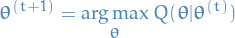 4
4
Notation
 is the
  observation
 is the rv. related to the
 - is a set of parameters for our model, which we want to estimate
- is the log-likelihood of the data given the estimated parameters
![$\underset{z^{ (i) } \sim Q_i}{E} [ \dots ]$](../../assets/latex/expectation_maximization_92b22dbb30ba20f2aff9ed0fb3fb320e0eb63fa1.png) means the expectation over the rv. using the probability distribution
means the expectation over the rv. using the probability distribution
Goal
- Have some model for

- Observe only

Objective is then to maximize:
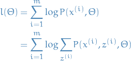 5
5
i.e. maximize the log-likelihood over the parameters
by marginalizing over
the rvs. .
Idea
The idea behind the EM algorithm is to at each step construct a lower-bound
for the log-likelihood using our estimate for from the previous
step. In this sense, the EM algorithm is a type of inference known as variational inference.
The reason for doing this is that we can often find a closed-form optimal value
for  , which is not likely to be the case if we simply
tried to take the derivative of
, which is not likely to be the case if we simply
tried to take the derivative of  set to zero and try to solve.
Finding the optimal parameters for the M-step is just to take the derivative of the
M-step, set to zero and solve. It turns out that this is more often easier than
directly doing the same for .
Viewing it in the form coordinate descent
If we let
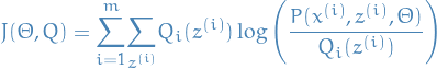 6
6
then we know from Jensen's inequality that  , and so increasing
  at each step also monotonically increases the log-likelihood . It can be shown that
this is then equivalent to using coordinate descent on
at each step also monotonically increases the log-likelihood . It can be shown that
this is then equivalent to using coordinate descent on  .
.
Derivation
If we take our objective defined above, we and simply multiply by
 , we get:
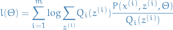 7
7
Where we choose to be s.t.  and
and  ,
i.e. is a probability distribution.
,
i.e. is a probability distribution.
We then observe that the last sum (within the  ) is actually the
following expectation:
) is actually the
following expectation:
![\begin{equation*}
\underset{z^{(i)}}{\sum} Q_i (z^{ (i) }) \frac{P(x^{ (i) }, z^{ (i) }, \Theta)}{Q_i (z^{ (i) })} =
\underset{z^{ (i) } \sim Q_i}{E} \Bigg[ \frac{P(x^{ (i) }, z^{ (i) }, \Theta)}{Q_i (z^{ (i) })} \Bigg]
\end{equation*}](../../assets/latex/expectation_maximization_13c626cfd74b1c8091ea10ec60d33f32a599778c.png) 8
8
Now using Jensen's inquality for a concave (because  is concave) function
  , which tells us
 ![$f(E[X]) \geq E[f(X)]$](../../assets/latex/expectation_maximization_e3025aae464d32e3c1aa1104a8897f1d7c98b121.png) :
:
![\begin{equation*}
\log \Bigg( \underset{z^{ (i) } \sim Q_i}{E} \Bigg[ \frac{P(x^{ (i) }, z^{ (i) }, \Theta)}{Q_i (z^{ (i) })} \Bigg] \Bigg) \geq
\underset{z^{ (i) } \sim Q_i}{E} \Bigg[ \log\Bigg( \frac{P(x^{ (i) }, z^{ (i) }, \Theta)}{Q_i (z^{ (i) })} \Bigg) \Bigg]
\end{equation*}](../../assets/latex/expectation_maximization_41f4e4c68fc58cabf1c5a10d1949a4658399dd03.png) 9
9
Thus, we have constructed a lower-bound on the log-likelihood:
![\begin{equation*}
l(\Theta) \geq \overset{m}{\underset{i=1}{\sum}} \underset{z^{ (i) } \sim Q_i}{E}
\Bigg[ \log\Bigg( \frac{P(x^{ (i) }, z^{ (i) }, \Theta)}{Q_i (z^{ (i) })} \Bigg) \Bigg]
\end{equation}x
Now what we want is for this inequality to be /tight/, i.e. that we have /equality/,
so that we ensure we're actually improving our estimate by each step.
Therefore we want to choose $Q_i$ s.t.
\begin{equation}
\frac{P(x^{ (i) }, z^{ (i) }, \Theta)}{Q_i (z^{ (i) })} = \text{constant}, \quad \forall z^{ (i) }
\end{equation*}](../../assets/latex/expectation_maximization_31802c2bbc63452c5130c8e77d07ad22b02e0bef.png) 10
10
Why? This would imply that the expectation above would also be constant. And since
![$f(c) = E[f(c)]$](../../assets/latex/expectation_maximization_a31b006b40ac40de6bcf4a10ea83fa618c248eec.png) is true for any constant
is true for any constant  , the inequality would be tight, i.e. be an equality, as wanted!
It's also equivalent of saying that we want to be proportional to 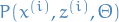 .
Combining this with the fact that we want to be a probability distribution, so we
need to satisfy the proportionality and
.
Combining this with the fact that we want to be a probability distribution, so we
need to satisfy the proportionality and  . Then it turns out (makes sense, since we need it to sum to 1 and be prop to
  )
that we want:
)
that we want:
 11
11
Which gives us the E-step of the EM-algorithm:
 12
12
Giving us a (tight) lower-bound for for the current estimate of .
The M-step is then to optimize that lower-bound wrt. :
 13
13
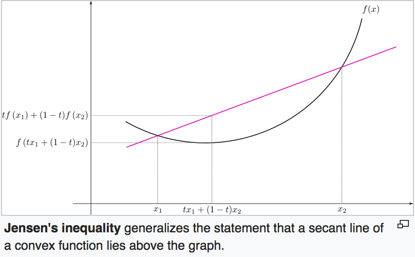
Appendix A: Jensen's inquality
If
- is a convex function.
 is a rv.
Then ![$f(E[X]) \leq E[f(x)]$](../../assets/latex/expectation_maximization_5a704c191584b112ce2eae76d3f11effcc23f4d9.png) .
.
Further, if  ( is strictly convex), then
![$E[(f(X)] = f(E[X]) \iff X = E[X]$](../../assets/latex/expectation_maximization_1a19363be0c70d388d505c858c79d669d8e4944c.png) "with probability 1".
"with probability 1".
If we instead have:
- is a concave function
Then . This is the one we need for the derivation of EM-algorithm.
To get a visual intuition, here is a image from Wikipedia: