Clustering algorithms
Table of Contents
Notation
 is the
  observation
 is the dimension of the data, i.e.
K-means clustering
Summary
- Guarantees local minima converges
- No guarantee for global minima
Notation
 is the mean of the cluster
Idea
K-means clustering is performing using two steps:
Randomly initialize
 cluster centroids with means
 1
1
Repeat until convergence:
- Set
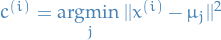 , i.e. assign the data
to the cluster for which it is closest to the mean.
, i.e. assign the data
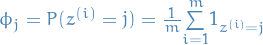
to the cluster for which it is closest to the mean. - Update mean of cluster as follows:
 μj = { {} 1 \{c(i) = j \} x(i)}
{{} 1 \{c(i) = j\} }
μj = { {} 1 \{c(i) = j \} x(i)}
{{} 1 \{c(i) = j\} }
- Set
Convergence here means until the assignments to the different clusters do not change.
Gaussian mixture models
Summary
Notation
 is the latent / unobserverd / hidden random variable which we want to estimate
 is the assigned cluster for the observation
  represents the probability of the
  "cluster" assignment
Idea
We have a latent random variable and  have a joint distribution:
 2
2
The model is as follows:
 where
where 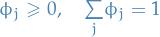
Note that this model is identical to Gaussian Discriminant Analysis, except the fact that we have replaced our labeled outputs
 by latent
variable .
by latent
variable .
Optimization
Special case of EM
See this for more on Expectation Maximization (EM).
Repeat until convergence:
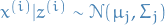
(E-step) Guess values of
's and compute:
 3
3
Where the
 means that we sum over the same expression as
in the numerator for every
means that we sum over the same expression as
in the numerator for every  , and the numerator is simply the Gaussian PDF
multiplied by the probability of
, and the numerator is simply the Gaussian PDF
multiplied by the probability of  .
.
- (M-step) Compute for each cluster :
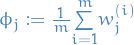 , i.e. take average of weights computed above
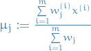 , i.e. weighted average for the ith observation
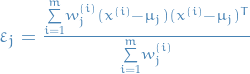 , i.e. the variance using the previously computed weights
Parallels to Gaussian Discriminant Analysis
In GDA we have:
But in our case (GMM) we do not know which cluster the observation
belongs to, so instead we use the "soft-weights"  and so get .
Mean-shift
- Non-parametric feature-space analysis technique for locating a maxima of a density function, a so-called mode-seeking algorithm
Mean shift is an iterative method for locating the maxima - the modes - of density function given discrete data sampled from that function.
- Choose a kernel function
 , which determines the weights of the nearby points for re-estimation of the mean.
 The weighted mean of the density in the window determined by
 is
is
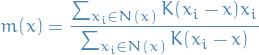
where
 is the neighborhood of
  , a set of points for which
  .
.
- Set

- Repeate 2-3 until
 converges
The procedure gets it's name from the difference  , which is called the mean shift.
A rigid proof for convergence of the algorithm using a general kernel in a high dimensional space is still not known.
Convergence has been shown for one-dimension with differentiable, convex, and strictly increasing profile function.
Convergence in higher dimensions with a finite number of the stationary points (or isolated) has been proven, however, sufficient conditions for a general kernel to have a finite (or isolated) stationary points have not been provided.