Gradient Boosting
Table of Contents
Gradient boosting
Overview
Gradient boosting is a technique for regression and classification problems, which produces a prediction model in the form of an ensemble of weak prediction models, typically prediction trees. It builds the model in a stage-wise fashion like other boosting methods do, and generalizes them by allowing optimization of an arbitrary differentiable loss function.
Motivation
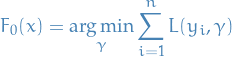
Consider a least-squares regression setting, where the goal is to "teach" a model  to predict values in the form
  by minimizing the mean squared error
  , averaged over some training set of actualy values of the output variable
  .
.
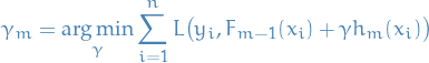
At each stage  , of gradient boosting, it may be assumed that there is a some imperfect model
  . The gradient boosing algorithm improves on by constructing a new model that adds an estimator
  to provide a better model:
  .
.
To find , the gradient boosting solution starts with the observation that a perfect would imply

i.e. that adding the extra predictor will make up for all the mistakes our previous model  did, or equivalently

Therefore, gradient boosting will fit to the residual  . Like in other boosting variants, each
  learns to correct its predecessor .
The generalization to other loss-functions than the least-squares, comes from the observation that for a given model are the negative gradients (wrt.  ) of the squared error loss function, hence for any loss function
  we'll simply fit to the negative gradient
  .
.
Algorithm
Input: training set  , a differentiable loss function
  , number of iterations
  .
.
Initialize model with a constant value:
For
 to :
to :
- Compute so-called psuedo-residuals :
![\begin{equation*}
r_{im} = - \Bigg[ \frac{\partial L(y_i, F(x_i))}{\partial F(x_i)} \Bigg]_{F(x) = F_{m-1}(x)} \quad \text{for } i = 1, \dots, n
\end{equation*}](../../assets/latex/boosting_bf5ab350fd8f28957deb4ae6d333d2aee3bd9983.png)
- Fit a base learner (e.g. tree) to psuedo-residuals, i.e. train it using the training set

- Compute multiplier
 sby solving the following one-dimension optimization problem
- Update the model:

- Output

Gradient Tree Boosting
- Uses decision trees of fixed size as base learners
Modified gradient boosting method ("TreeBoost")
- Generic gradient boosting at the m-th step would fit a decision tree
 to psuedo-residuals
 - Let
 be the number of its leaves
 Tree partitions input space into
disjoint regions  and predicts a constant value in each region, i.e.
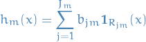
where
 is the value predicted in the region
  .
.
In the case of usual CART trees, where the trees are fitted using least-squares loss, and so the coefficient for the region is equal to just the value of the output variable, averaged over all training instances in .
Continuing with generic gradient boosting, the model is:
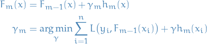
The modified gradient tree boosting ("TreeBoost") algorithm is then to instead choose a separate optimal value  for each of the tree's regions, instead of a single for whole tree:
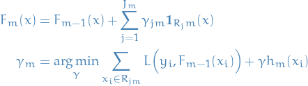
where we've simply absorbed into  .
.
Terminology
- Out-of-bag error / estimate is a method for measuring prediction error of methods utilizing bootstrap aggregating (bagging) to sub-sample data used for training.
OOB is the mean prediction error on each training sample
 , using only the trees that did not have in their bootstrap sample
Regularization
- Number of trees: Large number of trees can overfit
Shrinkage: use a modified update rule:

where
 is the learnin rate.
- Subsampling is when at each iteration of the algorithm, a base learner should be fit on a subsample of the training set drawn at random without replacement. Sumsample size
 is the fraction of training set to use; if
  then algorithm is deterministic and identitical to TreeBoost
 - Limit number of observations in trees' terminal nodes: in the tree building process by ignoring any split that lead to nodes containing fewer than this number of training set instances. Helps reduce variance in predictions at leaves.
- Penalize complexity of tree: model complexity can be defined as proportional number of leaves in the learned trees. Joint optimization of loss and model complexity corresponds to a post-pruning algorithm.
- Regularization (e.g.
 ,
,  ) on leaf nodes