RBM: Restricted Boltzmann Machines
Table of Contents
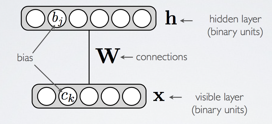
Overview
- One visible layer of observed binary units

- One hidden layer of unobserved binary units

Connections between every node in the different layers, i.e. restricted means no connections from hidden to hidden, nor from visible to visible, but connections between all hidden to visible pairs.
- Models Maximum Entropy distributions, and because of this, RBMs were originally motivated by Hinton as a "soft-constraint learner", where it was the intention that it would learn a distribution which satisfied the underlying constraints (see [BROKEN LINK: No match for fuzzy expression: *Principle%20of%20Maximum%20Entropy]).ackley_1985
Notation
 and
and  denotes visible units
- and
 denotes hidden units
  and
and  will used to denote bias of the visible units
 and
and  will be used to denote the bias of the hidden units
 denotes the empirical expectation
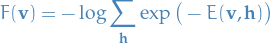
The so-called free-energy:
 and
and  denotes the t-th sample from a sampling chain for the visible and hidden variables, respectively.
 denote the vector but excluding the entry at index
  :
:

Factor graph view
A Boltzmann Machine is an energy-based model consisting of a set of hidden units  and a set of visible units
  , where by "units" we mean random variables, taking on the values and , respectively.
An Boltzmann Machine assumes the following joint probability distribution of the visible and hidden units:
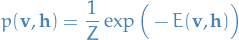
with  being the partition function (normalization factor) and the energy function

where  and
and  denote the convariance matrices for the visible and hidden units, respectively.
A Restricted Boltzmann Machine (RBM) is an energy-based model consisting of a set of hidden units and a set of visible units , whereby "units" we mean random variables, taking on the values and , respectively.
The restricted part of the name comes from the fact that we assume independence between the hidden units and the visible units, i.e.
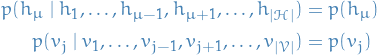
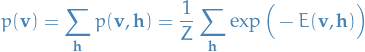
An RBM assumes the following joint probability distribution of the visible and hidden units:
with being the partition function (normalization factor) and the energy function
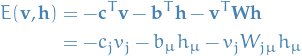
implicitly summing over repeating indices.
Training
Log-likelihood using gradient ascent
Notation
Used in the derivation of

Gradient of log-likelihood of energy-based models
RBMs assumes the following model
with

The minus-minus signs might seem redundant (and they are), but is convention due to the Boltzmann distribution found in physics.
where we're implicitly summing over repeating indices. First we observe that
Taking the log of this, we have
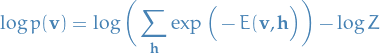
Now suppose we're given a set of samples  , then the likelihood (assuming i.i.d.) is given by
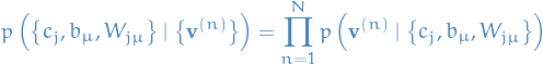
Taking the log of this expression, and using the above expression for  , we have
![\begin{equation*}
\begin{split}
\mathcal{L}(\big\{ c_j, b_{\mu}, W_{j \mu} \big\}) &= \sum_{n=1}^{N} \Bigg[ \log \bigg( \sum_{\mathbf{h}}^{} p \Big( \mathbf{v}^{(n)}, \mathbf{h} \Big) \bigg) - \log Z \Bigg] \\
&= \sum_{n=1}^{N} \Bigg[ \log \bigg( \sum_{\mathbf{h}}^{} p \Big( \mathbf{v}^{(n)}, \mathbf{h} \Big) \bigg) \Bigg] - N \log Z
\end{split}
\end{equation*}](../../assets/latex/restricted_boltzmann_machines_04ae14d4d2a1f8c0fa6ea9e1c9f524397f9f1601.png)
Let  , taking the partial derivative wrt.
  for the n-th term we have
![\begin{equation*}
\begin{split}
\frac{\partial }{\partial \theta} \Bigg[ \log \bigg( \sum_{\mathbf{h}}^{} p \Big( \mathbf{v}^{(n)}, \mathbf{h} \Big) - \log Z \Bigg] &= - \frac{\sum_{\mathbf{h}}^{} \frac{\partial E(\mathbf{v}, \mathbf{h})}{\partial \theta} p \Big( \mathbf{v}^{(n)}, \mathbf{h} \Big)}{\sum_{\mathbf{h}}^{} p \Big( \mathbf{v}^{(n)}, \mathbf{h} \Big)} - \frac{1}{Z} \frac{\partial Z}{\partial \theta}
\end{split}
\end{equation*}](../../assets/latex/restricted_boltzmann_machines_de58622643c4ccae2e581937d93975c4fb661dcc.png)
The first term can be written as an expectation
![\begin{equation*}
\frac{\sum_{\mathbf{h}}^{} \frac{\partial E(\mathbf{v}^{(n)}, \mathbf{h})}{\partial \theta} p \Big( \mathbf{v}^{(n)}, \mathbf{h} \Big)}{\sum_{\mathbf{h}}^{} p \Big( \mathbf{v}^{(n)}, \mathbf{h} \Big)} = \mathbb{E} \Bigg[ \frac{\partial E(\mathbf{v}^{(n)}, \mathbf{h})}{\partial \theta} \ \Big| \ \mathbf{v}^{(n)} \Bigg]
\end{equation*}](../../assets/latex/restricted_boltzmann_machines_39bf6562df22c7314d45556a14f8287415acbd95.png)
since on the LHS we're marginalizing over all and then normalizing wrt. the same distribution we just summed over.
For the second term recall that 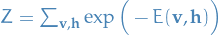 , therefore
![\begin{equation*}
\frac{1}{Z} \frac{\partial Z}{\partial \theta} = - \frac{1}{Z} \sum_{\mathbf{v}, \mathbf{h}}^{} \frac{\partial E(\mathbf{v}, \mathbf{h})}{\partial \theta} \exp \Big( - E(\mathbf{v}, \mathbf{h}) \Big) = - \mathbb{E} \Bigg[ \frac{\partial E(\mathbf{v}, \mathbf{h})}{\partial \theta} \Bigg]
\end{equation*}](../../assets/latex/restricted_boltzmann_machines_bf6639f2ff4cfe3174f6149fa82d9fa3143d5f8d.png)
Substituting it all back into the partial derivative of the log-likelihood, we end get
![\begin{equation*}
\frac{\partial \mathcal{L}}{\partial \theta} = - \sum_{n=1}^{N} \mathbb{E} \Bigg[ \frac{\partial E(\mathbf{v}^{(n)}, \mathbf{h})}{\partial \theta} \ \Bigg| \ \mathbf{v}^{(n)}\Bigg] + N \ \mathbb{E} \Bigg[ \frac{\partial E(\mathbf{v}, \mathbf{h})}{\partial \theta} \Bigg]
\end{equation*}](../../assets/latex/restricted_boltzmann_machines_6af6ac17fc4c097e1a78e82a6a18497d8ac72488.png)
Where the expectations are all over the probability distribution defined by the model.
Since maximizing  is equivalent to maximizing
  we instead consider
![\begin{equation*}
\frac{1}{N} \frac{\partial \mathcal{L}}{\partial \theta} = - \frac{1}{N} \sum_{n=1}^{N} \mathbb{E} \Bigg[ \frac{\partial E(\mathbf{v}^{(n)}, \mathbf{h})}{\partial \theta} \ \Bigg| \ \mathbf{v}^{(n)}\Bigg] + \mathbb{E} \Bigg[ \frac{\partial E(\mathbf{v}, \mathbf{h})}{\partial \theta} \Bigg]
\end{equation*}](../../assets/latex/restricted_boltzmann_machines_97fe9664498ddfcaca907d3e58dcbfdc1c62811e.png)
Dividing by  , observe that the first term can be written
![\begin{equation*}
\frac{1}{N} \sum_{n=1}^{N} \mathbb{E} \Bigg[ \frac{\partial E(\mathbf{v}^{(n)}, \mathbf{h})}{\partial \theta} \ \Bigg| \ \mathbf{v}^{(n)}\Bigg] = \left\langle \mathbb{E} \Bigg[ \frac{\partial E(\mathbf{v}, \mathbf{h})}{\partial \theta} \ \Bigg| \ \mathbf{v} \Bigg] \right\rangle_{\left\{ \mathbf{v}^{(n)} \right\}}
\end{equation*}](../../assets/latex/restricted_boltzmann_machines_47d83f2ebf9302b3e8ad95f47e5710548a221460.png)
Giving us
![\begin{equation*}
\frac{1}{N} \frac{\partial \mathcal{L}}{\partial \theta} = - \left\langle \mathbb{E} \Bigg[ \frac{\partial E(\mathbf{v}, \mathbf{h})}{\partial \theta} \ \Bigg| \ \mathbf{v} \Bigg] \right\rangle_{\left\{ \mathbf{v}^{(n)} \right\}} + \mathbb{E} \Bigg[ \frac{\partial E(\mathbf{v}, \mathbf{h})}{\partial \theta} \Bigg]
\end{equation*}](../../assets/latex/restricted_boltzmann_machines_0fba9d1b91434f37f7f0465c6961cfd330c2b990.png)
Clearly the second term is almost always intractable since we would have to sum over all possible and , but the first term might also be intractable as we would have to marginalize over all the hidden states with fixed to  .
.
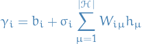
When working with binary hidden variables, i.e.  are all assumed to be Bernoulli random variables, then we have
![\begin{equation*}
\mathbb{E} [ \mathbf{h} \mid \mathbf{v} ] = \prod_{\mu = 1}^{|\mathcal{H}|} p(H_{\mu} = 1 \mid \mathbf{v})
\end{equation*}](../../assets/latex/restricted_boltzmann_machines_77cbec174af8e3bec4495660e71b4af0b9724a51.png)
In general, when the hiddens are not necessarily Bernoulli, we would also like to sample the hidden states to approximate the conditional expectation. It would make sense to sample some  number of hidden states for each observed , i.e.
![\begin{equation*}
\left\langle \mathbb{E} \Bigg[ \frac{\partial E(\mathbf{v}, \mathbf{h})}{\partial \theta} \ \Bigg| \ \mathbf{v} \Bigg] \right\rangle_{\left\{ \mathbf{v}^{(n)} \right\}} = \frac{1}{N} \sum_{n=1}^{N} \mathbb{E} \Bigg[ \frac{\partial E(\mathbf{v}^{(n)}, \mathbf{h})}{\partial \theta} \ \Bigg| \ \mathbf{v}^{(n)}\Bigg] \approx \frac{1}{N} \sum_{n=1}^{N} \frac{1}{M} \sum_{m=1}^{M} \frac{\partial E(\mathbf{v}^{(n)}, \mathbf{h}^{(m)})}{\partial \theta}
\end{equation*}](../../assets/latex/restricted_boltzmann_machines_1d6efc5d229a7d6dbbeae4fb738b7c2c91b7399f.png)
In fact, as mentioned on p.45 in Fischer_2015, this method (but letting  ) is often used, but, in the Bernoulli case, taking the expectation reduces the variance of our estimate compared to also sampling .
You will often see the notation
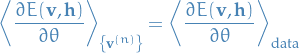
which we will use from now on. The  was used to make it explicit that we're computing the expectation over the visible units, NOT the joint expectation by sampling for each of the observed visible units.
For the second term we also use the empirical expectation as an approximation:
![\begin{equation*}
\mathbb{E} \Bigg[ \frac{\partial E(\mathbf{v}, \mathbf{h})}{\partial \theta} \Bigg] \approx \frac{1}{N} \frac{1}{M} \sum_{n=1}^{N} \sum_{m=1}^{M} \frac{\partial E(\mathbf{v}^{(n)}, \mathbf{h}^{(m)})}{\partial \theta}
\end{equation*}](../../assets/latex/restricted_boltzmann_machines_d99c16f62ca4a0a5898d4d55dd096e1224518f74.png)
Finally giving us a tractable approximation to the gradient of the log-likelihood:
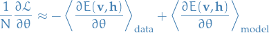
Making the variable takes on explicit, we have
Observe that the signs have switched, which is simply due to the fact that  depends negatively on all the variables
  .
.
Now we can make use of any nice stochastic gradient ascent method.
Bernoulli RBM
In the case of a Bernoulli RBM, both the visible and hidden variables only take on the values  . Therefore,
![\begin{equation*}
\begin{split}
\mathbb{E}\Big[h_{\mu} \mid \mathbf{v}^{(n)} \Big] &= 1 \cdot p\Big(H_{\mu} = 1 \mid \mathbf{v}^{(n)} \Big) + 0 \cdot p\Big(H_{\mu} = 0 \mid \mathbf{v}^{(n)} \Big) \\
&= p\Big(H_{\mu} = 1 \mid \mathbf{v}^{(n)} \Big)
\end{split}
\end{equation*}](../../assets/latex/restricted_boltzmann_machines_3d30cf5c1da881ad5ed19df865df66b3dc745119.png)
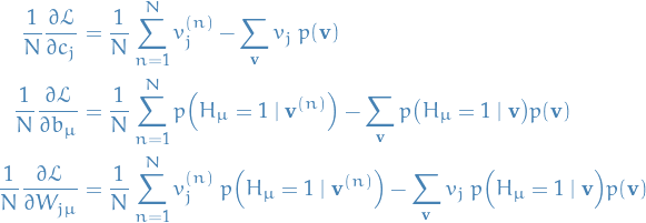
Hence, for the hidden units, we have
![\begin{equation*}
\left\langle h_{\mu} \right\rangle_{\text{data}} = \frac{1}{N} \sum_{n=1}^{N} \mathbb{E} \Big[ h_{\mu} \mid \mathbf{v}^{(n)} \Big] = \frac{1}{N} \sum_{n=1}^{N} p \Big( H_{\mu} = 1 \mid \mathbf{v}^{(n)} \Big)
\end{equation*}](../../assets/latex/restricted_boltzmann_machines_c6ad0ae2a707b7d49d89ef213d2cbb5a68a1e906.png)
and
![\begin{equation*}
\left\langle h_{\mu} \right\rangle_{\text{model}} = \mathbb{E}[h_{\mu}] = \sum_{\mathbf{v}}^{} p \Big( H_{\mu} = 1 \mid \mathbf{v}\Big) p (\mathbf{v} )
\end{equation*}](../../assets/latex/restricted_boltzmann_machines_b9c1aab93a23ffe50770f00ffd2cf0b269a35bb0.png)
For the visible units we have
![\begin{equation*}
\left\langle v_j \right\rangle_{\text{data}} = \frac{1}{N} \sum_{n=1}^{N} \mathbb{E}\Big[ v_j \mid \mathbf{v}^{(n)} \Big] = \frac{1}{N} \sum_{n=1}^{N} v_j^{(n)}
\end{equation*}](../../assets/latex/restricted_boltzmann_machines_9664634318a0d9426a9c21df9eeca6d67d9cc16f.png)
and
![\begin{equation*}
\left\langle v_j \right\rangle_{\text{model}} = \mathbb{E}[v_j] = \sum_{\mathbf{v}}^{} v_j \ p(\mathbf{v})
\end{equation*}](../../assets/latex/restricted_boltzmann_machines_970e03dd92b24ac64ea5bf7c36ff8f1d4db1dff6.png)
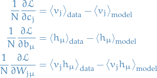
Thus, we end up with the gradients of the negative log-likelihood
In these expressions, the first terms are indeed tractable but the second terms still pose a problem. Therefore we turn to MCMC methods for estimating the expectations in the second terms.
A good method would (block) Gibbs sampling, since the visible and hidden units are independent, and we could thus sample all the visible or hidden units simultaneously. To obtain unbiased estimates we would then run the sampler for a large number of steps. Unfortunately this is expensive, which is where Contrastive Divergence comes in.
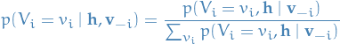
Expression for 
Let denote the vector but excluding the entry at index , then
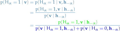
where in the last step we simply marginalize of  .
.
The numerator will be the exponential of the following three terms added together
and the denominator will be
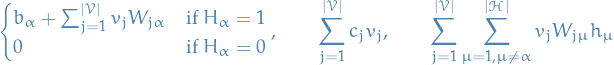
To be explicit, the denominator is

which we can write
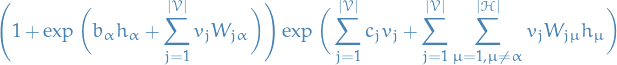
Taking the logarithm (for readability's sake), we end up with
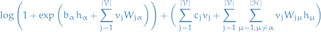
Hence,
![\begin{equation*}
\begin{split}
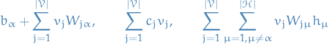
\log p \big( H_{\alpha} = 1 \mid \mathbf{v} \big) =& \quad \textcolor{green}{\Bigg[ b_{\alpha} + \sum_{j=1}^{|\mathcal{V}|} v_j W_{j \alpha} + \sum_{j=1}^{|\mathcal{V}|} c_j v_j + \sum_{j=1}^{|\mathcal{V}|} \sum_{\mu = 1, \mu \ne \alpha}^{|\mathcal{H}|} v_j W_{j \mu} h_{\mu}\Bigg]} \\
& - \textcolor{blue}{\Bigg[ \log \Bigg( 1 + \exp \bigg( b_{\alpha} h_{\alpha}
+ \sum_{j=1}^{|\mathcal{V}|} v_j W_{j \alpha} \bigg) \Bigg)
+ \bigg( \sum_{j=1}^{|\mathcal{V}|} c_j v_j + \sum_{j=1}^{|\mathcal{V}|} \sum_{\mu = 1, \mu \ne \alpha}^{|\mathcal{H}|} v_j W_{j \mu} h_{\mu}\bigg) \Bigg]}
\end{split}
\end{equation*}](../../assets/latex/restricted_boltzmann_machines_f63f8c5c067cf58f14d96961777aedb6d1cb078a.png)
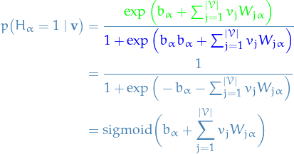
Observe that the two last terms in these expression cancels each other, thus
![\begin{equation*}
\log p \big( H_{\alpha} = 1 \mid \mathbf{v} \big) = \textcolor{green}{\Bigg[ b_{\alpha} + \sum_{j=1}^{|\mathcal{V}|} v_j W_{j \alpha} \Bigg]}
- \textcolor{blue}{\Bigg[ \log \Bigg( 1 + \exp \bigg( b_{\alpha} h_{\alpha} + \sum_{j=1}^{|\mathcal{V}|} v_j W_{j \alpha} \bigg) \Bigg) \Bigg]}
\end{equation*}](../../assets/latex/restricted_boltzmann_machines_fa9c36599facd78fccfc45e88622b7eb4ff7f652.png)
Finally, taking the exponential again,
TODO Computing
Gaussian RBM
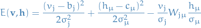
Suppose now that  are now continuous variables but are still bernoulli. We assume the following Hamiltonian / energy function
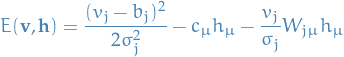
where, as usual, we assume summation over the repeated indices.
 denotes the variance of
 - We use the term
 in the "covariance" term, as it makes sense to remove the variance in which does not arise due to its relationship with the hiddens.
Computing and 
First observe that

And,
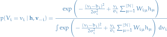
We know that
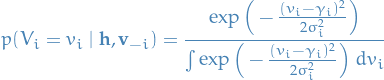
![\begin{equation*}
\begin{split}
p(V_i = v_i, \mathbf{h} \mid \mathbf{v}_{-i})
&= \exp \Big( - E(v_i, \mathbf{v}_{-i}, \mathbf{h}) \Big) \\
&= \exp \Bigg[ \Bigg( - \frac{(v_i - b_i)^2}{2 \sigma_i^2} + \sum_{\mu = 1}^{|\mathcal{H}|} \frac{v_i}{\sigma_i} W_{i \mu} h_{\mu} \Bigg) + \\
& \qquad \quad \Bigg( \sum_{j=1, j \ne i}^{|\mathcal{V}|}- \frac{(v_j - b_j)^2}{2 \sigma_j^2} + \frac{v_j}{\sigma_j} \sum_{\mu = 1}^{|\mathcal{H}|} W_{j \mu} h_{\mu} + \sum_{\mu = 1}^{|\mathcal{H}|} c_{\mu} h_{\mu} \Bigg) \Bigg]
\end{split}
\end{equation*}](../../assets/latex/restricted_boltzmann_machines_6efb261a86229817ce1fcb6f7c40d53b6ad90636.png)
where we've separated the terms depending on  and
and  . Why? In the denominator, we're integrating over all possible values of , hence any factor not dependent on we can move out of the integral. And since we find the same factor in the numerator, we can simply cancel the second term in the above expression. This leaves us with
Now, writing out the term in the exponent,
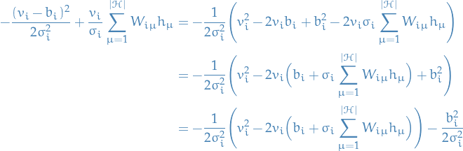
For readability's sake, let
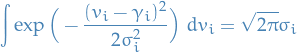
Then we can "complete the square" in the first term, which gives us

Finally, subsituting this back into our expression for  , keeping in mind that
  does not depend on and can therefore pulled out of the integral, we get
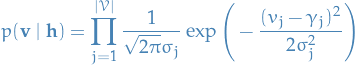
where we've cancelled the exponentials of  due to the independence mentioned above. But HOLD ON; these exponentials are simply Gaussians with mean !, hence
Thus,
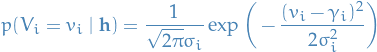
Or equivalently,
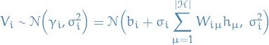
And we now understand why we call the resulting RBM of using this specific energy function a Gaussian RBM!
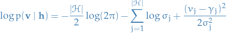
A final note is that
due to the independence the visible units conditioned on the hidden units, as usual in an RBM. Hence
Or more numerically more conveniently,
- What if also are Gaussian?
What happens if we instead have the following energy function
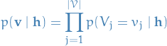
Going back to our expression for the distribution of

The only dependence on
arises from the multiplication with  in the energy function, hence the distribution of the visible units when the hidden can also take on continuous values, is simply
The only addition being the factor of
 in the sum.
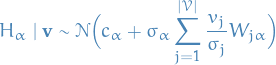
What about ?
Looking at our derivation for , the derivation for the hiddens given the visibles is exactly the same, substituting  with
with  and
and  with , giving us
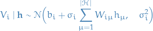
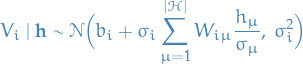
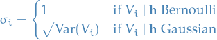
General expressions for both Bernoulli and Gaussians
If you've had a look at the derivations for the conditional probabilties and when and are Bernoulli or Gaussian, you might have observed that the expressions in the exponentials are very similar. In fact, we have the following
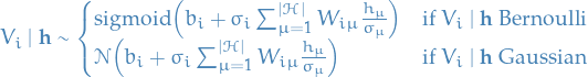
with
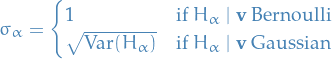
and for the hiddens
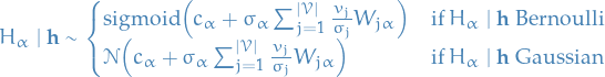
with
If we want to implement an RBM, allowing the possibility of using both Bernoulli and Gaussian hidden and / or visible units, we can!
Still need to make appropriate corrections in the free energy computation, i.e. when computing  .
.
Contrastive Divergence (CD)
The idea of Contrastive Divergence is to approximate the gradient of the log-likelihood we saw earlier
by
- Initialize "gradients"

- For
 :
:
- Initialize sampler with training instance (instead of using a random initialization)
- For
 do
do
 , where entries are of course independent of each other (due to biparite structure of an RBM)
 , where entries are of course independent of each other (due to biparite structure of an RBM)
- Compute gradients replacing with .

- Initialize sampler with training instance
Update parameters:

where
is the learning rate
![\begin{algorithm*}[H]\label{alg:contrastive-divergence}
\KwData{Observations of the visible units: $\{ \mathbf{v}^{(n)}, n = 1, \dots, N \}$}
\KwResult{Estimated parameters for an RBM: $(\mathbf{b}, \mathbf{c}, \mathbf{W})$}
$b_j := 0$ for $j = 1, \dots, |\mathcal{V}|$ \\
$c_{\mu} := 0$ for $\mu = 1, \dots, |\mathcal{H}|$ \\
$W_{j\mu} \sim \mathcal{N}(0, 0.01)$ for $(j, \mu) \in \left\{ 1, \dots, |\mathcal{V}| \right\} \times \left\{ 1, \dots, |\mathcal{H}| \right\}$ \\
\While{not converged}{
$\Delta b_j := 0$ \\
$\Delta c_{\mu} := 0$ \\
$\Delta W_{j \mu} := 0$ \\
\For{$n = 1, \dots, N$}{
\tcp{initialize sampling procedure}
$\hat{\mathbf{v}} := \mathbf{v}^{(n)}$ \\
\tcp{sample using Gibbs sampling}
\For{$t = 1, \dots, k$}{
$\hat{\mathbf{h}} \sim p(\mathbf{h} \mid \hat{\mathbf{v}})$ \\
$\hat{\mathbf{v}} \sim p(\mathbf{v} \mid \hat{\mathbf{h}})$
}
\tcp{accumulate changes}
$\Delta b_j \leftarrow \Delta b_j + v_j^{(n)} - \hat{v}_j$ \\
$\Delta c_{\mu} \leftarrow \Delta c_{\mu} + p\big(H_{\mu} = 1 \mid \mathbf{v}^{(n)} \big) - p \big( H_{\mu} = 1 \mid \hat{\mathbf{v}} \big)$ \\
$\Delta W_{j \mu} \leftarrow \Delta W_{j \mu} + v_j^{(n)} p\big(H_{\mu} = 1 \mid \mathbf{v}^{(n)} \big) - \hat{v}_j p \big( H_{\mu} = 1 \mid \hat{\mathbf{v}} \big)$ \\
}
\tcp{update the parameters of the RBM using average gradient}
$b_j \leftarrow b_j + \frac{\Delta b_j}{N}$ \\
$h_{\mu} \leftarrow h_{\mu} + \frac{\Delta h_{\mu}}{N}$ \\
$W_{j \mu} \leftarrow W_{j \mu} + \frac{\Delta W_{j \mu}}{N}$ \\
}
\caption{\textbf{Contrastive Divergence (CD-k)} with $k$ sampling steps.}
\end{algorithm*}](../../assets/latex/restricted_boltzmann_machines_d186d18367ae658df1f00c264c07ad6b66db9b37.png) 1
1
This is basically the algorithm presented in Fischer_2015, but in my opinion this ought to be the average gradient, not the change summed up. Feel like there is a factor of  missing here.
Of course, one could just absorb this into the learning rate, as long as the number of samples in each batch is the same.
Why not compute the expectation as one samples these  steps, why only do it at the end of the chain?
That is, when performing the approximation for the log-likelihood for a single training example
![\begin{equation*}
\frac{\partial \log p(\mathbf{v}^{(n)})}{\partial \theta} \approx - \frac{\partial F(\mathbf{v})}{\partial \theta} + \mathbb{E}_{\tilde{\mathbf{v}}^{(k)}} \bigg[ \frac{\partial F(\mathbf{v})}{\partial \theta} \ \Big| \ \mathbf{v}^{(n)} \bigg]
\end{equation*}](../../assets/latex/restricted_boltzmann_machines_29e1543083edef3d873e7ce040ea313ee600e445.png)
by replacing the expectation by sampling  , i.e.
![\begin{equation*}
\mathbb{E}_{\tilde{\mathbf{v}}^{(k)}} \bigg[ \frac{\partial F(\mathbf{v})}{\partial \theta} \ \Big| \ \mathbf{v}^{(n)} \bigg] \approx \frac{\partial F(\tilde{\mathbf{v}}^{(k)})}{\partial \theta}
\end{equation*}](../../assets/latex/restricted_boltzmann_machines_4148bf56c0539d8e864564a27f86ecd6f228a29c.png)
where  denotes the t-th sample from a sampler chain, initialized by the training example .
This leaves us with the update rule (for a single training example):
Why not compute the expectation over all these steps? Instead of stochastically approximating this expectation by a single example (the final sample in the chain), we could use the following approximation to the expectation
![\begin{equation*}
\mathbb{E}_{\tilde{\mathbf{v}}^{(k)}} \bigg[ \frac{\partial F(\mathbf{v})}{\partial \theta} \ \Big| \ \mathbf{v}^{(n)} \bigg] = \frac{1}{k} \sum_{t=1}^{k} \frac{\partial F(\tilde{\mathbf{v}}^{(t)})}{\partial \theta}
\end{equation*}](../../assets/latex/restricted_boltzmann_machines_33ddcd7932a9591e7174e6c61d747256990504b4.png)
I guess some reasons could be:
- more biased estimate (the more steps we let the sampler take, the more likely our sample is to be unbiased)
- more expensive to compute gradient than sampling
Theoretical justification
Most, if not all, is straight up copied from bengio_2009.
Consider a Gibbs chain  starting at a data point, i.e.
  for some
  .
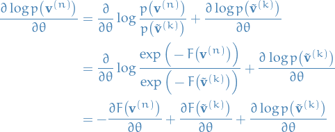
Then the log-likelihood at any step
.
Then the log-likelihood at any step  of the chain can be written
and since this is true for any path,
![\begin{equation*}
\log p \big( \mathbf{v}^{(n)} \big) = \mathbb{E}_{\tilde{\mathbf{v}}^{(k)}} \Bigg[ \log \frac{p \big( \mathbf{v}^{(n)} \big)}{p \big( \tilde{\mathbf{v}}^{(k)} \big)} \ \Big| \ \mathbf{v}^{(n)} \Bigg] + \mathbb{E}_{\tilde{\mathbf{v}}^{(k)}} \Big[ \log p \big( \tilde{\mathbf{v}}^{(k)} \mid \mathbf{v}^{(n)} \big) \Big]
\end{equation*}](../../assets/latex/restricted_boltzmann_machines_44cea7f2e07e2688c8de1588b4e46f72c95ff00e.png)
where the expectations are over Markov chain sample paths, conditioned on the starting sample .
The first equation is obvious, while the second equation requires rewriting
and substituting in the first equation.
For any model  with parameters
![\begin{equation*}
\mathbb{E} \Bigg[ \frac{\partial p(\mathbf{y})}{\partial \theta} \Bigg] = 0
\end{equation*}](../../assets/latex/restricted_boltzmann_machines_ced103a7e4a514070540951e6c983d9e3b834f9e.png)
when the expected value is taken accordin to .
![\begin{equation*}
\begin{split}
\mathbb{E} \Bigg[ \frac{\partial p(\mathbf{y})}{\partial \theta} \Bigg] &= \sum_{\mathbf{y}}^{} p(\mathbf{y}) \frac{\partial \log p(\mathbf{y})}{\partial \theta} \\
&= \sum_{\mathbf{y}}^{} \frac{p(\mathbf{y})}{p(\mathbf{y})} \frac{\partial p(\mathbf{y})}{\partial \theta} \\
&= \frac{\partial }{\partial \theta} \sum_{\mathbf{y}}^{} p(\mathbf{y}) \\
&= \frac{\partial }{\partial \theta} 1 = 0
\end{split}
\end{equation*}](../../assets/latex/restricted_boltzmann_machines_215cbdfd0efbb24b3f0716ed3f12869f27fe897a.png)
(Observe that for this to work with continuous variables we need to ensure that we're allowed to interchange the partial derivative and the integration symbol)
Consider a Gibbs chain starting at a data point, i.e. for some .
The log-likelihood gradient can be written
![\begin{equation*}
\frac{\partial \log p \big( \mathbf{v}^{(n)} \big)}{\partial \theta} = - \frac{\partial F \big( \mathbf{v}^{(n)} \big)}{\partial \theta} + \mathbb{E} \Bigg[ \frac{\partial F \big( \tilde{\mathbf{v}}^{(k)} \big)}{\partial \theta} \ \Big| \ \mathbf{v}^{(n)} \Bigg] + \mathbb{E}_{\tilde{\mathbf{v}}^{(k)}} \Bigg[ \frac{\partial \log p \big( \tilde{\mathbf{v}}^{(k)} \big)}{\partial \theta} \ \Big| \ \mathbf{v}^{(n)} \Bigg]
\end{equation*}](../../assets/latex/restricted_boltzmann_machines_d70ae54e986a49fb3c8b285cbb5aea43ecaf9ea8.png)
and
![\begin{equation*}
\lim_{k \to \infty} \mathbb{E}_{\tilde{\mathbf{v}}^{(k)}} \Bigg[ \frac{\partial \log p \big( \tilde{\mathbf{v}}^{(k)} \big)}{\partial \theta} \ \Big| \ \mathbf{v}^{(n)} \Bigg] = 0
\end{equation*}](../../assets/latex/restricted_boltzmann_machines_5d239ec71a57a6f7dc5b3a4c0757ab704c7e49c6.png)
Taking the derivative of the expression in Lemma 1, we get
Taking the expectations wrt. the Markov chain conditional on , we get
![\begin{equation*}
\frac{\partial \log p\big( \mathbf{v}^{(n)} \big)}{\partial \theta} = - \frac{\partial F \big( \mathbf{v}^{(n)} \big)}{\partial \theta} + \mathbb{E}_{\tilde{\mathbf{v}}^{(k)}} \Bigg[ \frac{\partial F \big( \tilde{\mathbf{v}}^{(k)} \big)}{\partial \theta} \ \Big| \ \mathbf{v}^{(n)} \Bigg] + \mathbb{E}_{\tilde{\mathbf{v}}^{(k)}} \Bigg[ \frac{\partial \log p \big( \tilde{\mathbf{v}}^{(k)} \big)}{\partial \theta} \ \Big| \ \mathbf{v}^{(n)} \Bigg]
\end{equation*}](../../assets/latex/restricted_boltzmann_machines_88a0ccab59b0bd864bfea4d9c924a5ebc7d0ccaf.png)
To show that the last term vanishes for  , we use the assumed convergence of the chain, which can be written

with
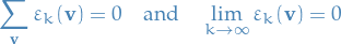
We can then rewrite the last expectation as
![\begin{equation*}
\begin{split}
\mathbb{E}_{\tilde{\mathbf{v}}^{(k)}} \Bigg[ \frac{\partial \log p \big( \tilde{\mathbf{v}}^{(k)} \big)}{\partial \theta} \ \Big| \ \mathbf{v}^{(n)}\Bigg]
&= \sum_{\tilde{\mathbf{v}}^{(k)}}^{} p \big( \tilde{\mathbf{v}}^{(k)} \mid \mathbf{v}^{(n)} \big) \frac{\partial \log p \big( \tilde{\mathbf{v}}^{(k)} \big)}{\partial \theta} \\
&= \sum_{\tilde{\mathbf{v}}^{(k)}}^{} \Big( p \big( \tilde{\mathbf{v}}^{(k)} \big) + \varepsilon_k \big( \tilde{\mathbf{v}}^{(k)} \big) \Big) \frac{\partial \log p \big( \tilde{\mathbf{v}}^{(k)} \big)}{\partial \theta} \\
&= \sum_{\tilde{\mathbf{v}}^{(k)}}^{} p \big( \tilde{\mathbf{v}}^{(k)} \big) \frac{\partial \log p \big( \tilde{\mathbf{v}}^{(k)} \big)}{\partial \theta} + \sum_{\tilde{\mathbf{v}}^{(k)}}^{} \varepsilon_k \big( \tilde{\mathbf{v}}^{(k)} \big) \frac{\partial \log p \big( \tilde{\mathbf{v}}^{(k)} \big)}{\partial \theta}
\end{split}
\end{equation*}](../../assets/latex/restricted_boltzmann_machines_78c9331ea2027722e38ff5ef5fc54e921500c745.png)
Using Lemma 2, the first sum vanishes, and we're left with
![\begin{equation*}
\begin{split}
\left| \mathbb{E}_{\tilde{\mathbf{v}}^{(k)}} \Bigg[ \frac{\partial \log p \big( \tilde{\mathbf{v}}^{(k)} \big)}{\partial \theta} \ \Big| \ \mathbf{v}^{(n)} \Bigg] \right|
&\le \sum_{\tilde{\mathbf{v}}^{(k)}}^{} \left| \varepsilon_k \big( \tilde{\mathbf{v}}^{(k)} \big) \right| \left| \frac{\partial \log p \big( \tilde{\mathbf{v}}^{(k)} \big)}{\partial \theta} \right| \\
&\le \Bigg( N_{\mathbf{v}} \max_{\mathbf{v}} \left| \frac{\partial \log p \big( \mathbf{v} \big)}{\partial \theta} \right| \Bigg) \varepsilon_k
\end{split}
\end{equation*}](../../assets/latex/restricted_boltzmann_machines_e2158b526b0b18a8c9553669cb8cc30dae09ff2e.png)
where  denotes the number of possible discrete configurations
  can take on, and we've let
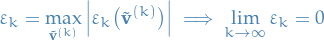
Hence this expectation goes to zero, completing our proof.
The proof above also tells us something important: the error due to the second expectation in CD-k has an upper bound which depends linearly on the sampler-error  .
.
Therefore the mixing-rate of the chain is directly related to the error of CD-k.
(Important to remember that there is of course also errors introduced in the stochastic approximation to the first part of the expectation too.)
Persistent Contrastive Divergence (PCD)
Persistent Contrastive Divergence (PCD) is obtained from CD approximation by replacing the sample  by a sample from a Gibbs chain that is independent of the sample
  of the training distribution.
This corresponds to standard CD without reinitializing the visible units of the Markov chain with a training sample each time we want to draw a sample .
![\begin{algorithm*}[H]\label{alg:persistent-contrastive-divergence}
\KwData{Observations of the visible units: $\{ \mathbf{v}^{(n)}, n = 1, \dots, N \}$}
\KwResult{Estimated parameters for an RBM: $(\mathbf{b}, \mathbf{c}, \mathbf{W})$}
$b_j := 0$ for $j = 1, \dots, |\mathcal{V}|$ \\
$c_{\mu} := 0$ for $\mu = 1, \dots, |\mathcal{H}|$ \\
$W_{j\mu} \sim \mathcal{N}(0, 0.01)$ for $(j, \mu) \in \left\{ 1, \dots, |\mathcal{V}| \right\} \times \left\{ 1, \dots, |\mathcal{H}| \right\}$ \\
\While{not converged}{
$\Delta b_j := 0$ \\
$\Delta c_{\mu} := 0$ \\
$\Delta W_{j \mu} := 0$ \\
\tcp{initialize sampling procedure BEFORE training loop}
$\hat{\mathbf{v}} := \mathbf{v}^{(n)}$ for some $n \in \left\{ 1, \dots, N \right\}$ \\
\For{$n = 1, \dots, N$}{
\tcp{sample using Gibbs sampling}
\tcp{using final sample from previous chain as starting point}
\For{$t = 1, \dots, k$}{
$\hat{\mathbf{h}} \sim p(\mathbf{h} \mid \hat{\mathbf{v}})$ \\
$\hat{\mathbf{v}} \sim p(\mathbf{v} \mid \hat{\mathbf{h}})$
}
\tcp{accumulate changes}
$\Delta b_j \leftarrow \Delta b_j + v_j^{(n)} - \hat{v}_j$ \\
$\Delta c_{\mu} \leftarrow \Delta c_{\mu} + p\big(H_{\mu} = 1 \mid \mathbf{v}^{(n)} \big) - p \big( H_{\mu} = 1 \mid \hat{\mathbf{v}} \big)$ \\
$\Delta W_{j \mu} \leftarrow \Delta W_{j \mu} + v_j^{(n)} p\big(H_{\mu} = 1 \mid \mathbf{v}^{(n)} \big) - \hat{v}_j p \big( H_{\mu} = 1 \mid \hat{\mathbf{v}} \big)$ \\
}
\tcp{update the parameters of the RBM using average gradient}
$b_j \leftarrow b_j + \frac{\Delta b_j}{N}$ \\
$h_{\mu} \leftarrow h_{\mu} + \frac{\Delta h_{\mu}}{N}$ \\
$W_{j \mu} \leftarrow W_{j \mu} + \frac{\Delta W_{j \mu}}{N}$ \\
}
\caption{\textbf{Persistent Contrastive Divergence (PCD-k)} with $k$ steps. Initialize next chain from final state of previous chain.}
\end{algorithm*}](../../assets/latex/restricted_boltzmann_machines_ba11e891397ef63d73bf79b725b132bddb560e53.png) 1
1
Parallel Tempering (PT)
Parallel Tempering (PT) introduces supplementary Gibbs chains that sample from more and more smoothed replicas of the original distribution.
Formally, given an ordered set of temperatures  , and we define a set of Markov chains with stationary distributions
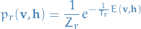
for  where
where  is the corresponding partition function, and
  has exactly the model distribution.
- With increasing temperature,
 becomes more and more equally distribution
 - As
 we have
  , i.e. uniform distribution
- Subsequent samples of the Gibbs chain are independent of each other, thus stationary distribution is reached after just one sampling step
In each step of the algorithm, we run Gibbs sampling steps in each tempered Markov chain yielding samples  .
.
Then, two neighboring Gibbs chains with temperatures  and
and  may exchange "particles"
  and
and  with probability (based on Metropolis ratio),
which gives, for RBMs,
![\begin{equation*}
\min \left\{ 1, \exp \Bigg[ \Bigg( \frac{1}{T_r} - \frac{1}{T_{r - 1}} \Bigg) \bigg( E(\mathbf{v}_r, \mathbf{h}_r) - E(\mathbf{v}_{r - 1}, \mathbf{h}_{r - 1}) \bigg) \Bigg] \right\}
\end{equation*}](../../assets/latex/restricted_boltzmann_machines_34d6b065495c3005112d20d3b7aefeb637a52fcf.png)
After performing these "swaps" between chains (which increase the mixing rate), we take the sample  from the original chain with
  as the sample from RBM distribution.
This procedure is repeated  times, yielding the samples
  used for the approximation of the expectation under the RBM distribution in the log-likelihood gradient. Usually is the number of samples in the batch of training data.
Compared to CD, PT produces more quickly mixing Markov chain, thus less biased gradient approximation, at the cost of computation.
Estimating partition function
Bibliography
Bibliography
- [ackley_1985] Ackley, Hinton, & Sejnowski, A Learning Algorithm for Boltzmann Machines*, Cognitive Science, 9(1), 147–169 (1985). link. doi.
- [Fischer_2015] Fischer, Training Restricted Boltzmann Machines, KI - Künstliche Intelligenz, 29(4), 441–444 (2015). link. doi.
- [bengio_2009] Bengio & Delalleau, Justifying and Generalizing Contrastive Divergence, Neural Computation, 21(6), 1601–1621 (2009). link. doi.