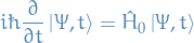
Quantum Mechanics
Table of Contents
- Reading
- Progress
- Definitions
- Stuff
- Zero point energy
- Quantum Harmonic Oscillator
- Correspondance principle
- Operators
- Coherence
- Observables
- Momentum
- Angular momentum
- Angular momentum - reloaded
- Central potential
- Hydrogen atom
- Spin - intrinsic angular momentum
- Addition of angular momenta
- Identical Particles
- Fourier Transforms and Uncertainty Relations
- Bra, kets, and matrices
- Time-independent Perturbation Theory
- Time-dependent Perturbation Theory
- Radiation
- Quantum Scattering Theory
- Central Field Approximation
- Variational Method
- Hidden Variables, EPR Paradox, Bell's Inequality
- Quantum communication
- Quantum computing
- Cohen-Tannoudji - Quantum Mechanics
- Principles of Quantum Mechanics - Dirac
- Quantum Theory for Mathematicians
- Notation
- 2. A First Approach to Classical Mechanics
- 3. A First Approach to Quantum Mechanics
- 4. The Free Schrödinger Equation
- 5. A Particle in a Square Well
- 6. Perspectives on the Spectral Theorem
- 7. Spectral Theorem for Bounded Self-Adjoint Operators
- 8. Spectral Theorem for Bounded Self-Adjoint Operators: Proofs
- Practice problems
- Q & A
Reading
- Quantum Physics - Stephen Gasiorowicz
- "Quantum Physics", Messiah, p. 463 Appendix A: Distributions & Fourier Transform
Progress
- Note taken on
p. 115
Definitions
Words
- plane wave
- multi-dimensional wave
- wave packet
- superposition of plane waves
- hilbert space
- Banach space withe addition of an inner product
- banach space
- Space with metric, and is complete wrt. to the metric in a sense that each Cauchy sequence converges to a limit within the space.
- isotropic
- Independent of orientation.
Bound / unbound wave equations
Bound energy
Restricts us to positive energies 
Unbound energy
Allows both positive and negative energies 
Schrödinger equation
Operators
Position operator

Russel-Sanders notation
States that arise in coupling orbital angular momentum  and spin
  to give total angular momentum
  are denoted:

where the  is "optional" (not always included).
Further, remember that we often use the following notation to denote the different angular momentum :

Stuff
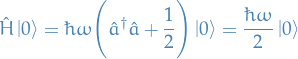
Zero point energy
Heisenbergs uncertainty principle tells us that a particle cannot sit motionless at the bottom of it's potential well, as this would imply that the uncertainty in momentum  would be infinite. Therefore, the lowest-energy state of the system (called ground state ) must be a distribution for the position and momentum which at all times satisfy the uncertainty principle.
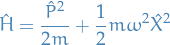
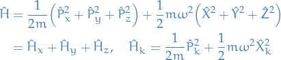
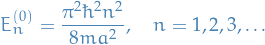
Near the bottom of a potential well, the Hamiltonian of a general system (the quantum-mechanical operator giving a system its energy) can be approximated as a quantum harmonic oscillator:
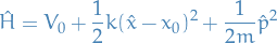
Quantum Harmonic Oscillator
![\begin{equation*}
\hat{H} = \Bigg[ - \frac{\hbar^2}{2m} \frac{\partial^2}{\partial x^2} + \frac{1}{2} m \omega^2 x^2 \Bigg]
\end{equation*}](../../assets/latex/quantum_mechanics_7c9244b8b792fc892f30045f30726f21b7065032.png)
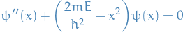
Thus, the eigenvalue function of the Hamiltonian becomes
![\begin{equation*}
\Bigg[ - \frac{\hbar^2}{2m} \frac{\partial^2}{\partial x^2} + \frac{1}{2} m \omega^2 x^2 \Bigg] \psi = E \psi
\end{equation*}](../../assets/latex/quantum_mechanics_2f748733cb811a4375991e37f90dfb46653a92b6.png)
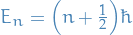
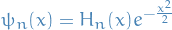
As it turns out, this differential equation has the eigenfunctions:
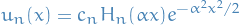
where  denote the n-th [BROKEN LINK: No match for fuzzy expression: *Hermite%20polynomials], with
  .
.
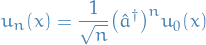
Further, using the raising and lowering operators discussed in Angular momentum - reloaded we can rewrite the solutions as
Annihiliation / lowering operator:
Creation / Raising operator:
Solution
There's two ways of going about this:
- Solving using the ladder operators, but you somehow need to obtain the ground levels
- Solving using straight up good ole' method of variation of parameters and Sturm-Liouville theory
Solving using ladder-operators
- Notation
 is the eigenfunction corresponding to the n-th eigenvalue
 , which is dimensionless
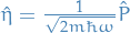 , which is dimensionless

- Stuff
The Hamiltonian in this case is given by
with the TISE

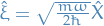
For convenience we rewrite the Hamiltonian
![\begin{equation*}
\begin{split}
\hat{H} &= \hbar \omega \Bigg[ \frac{\hat{P}^2}{2 m \hbar \omega} + \frac{m \omega}{2 \hbar} \hat{X}^2 \Bigg] \\
&= \hbar \omega \Big[ \hat{\eta}^2 + \hat{\xi}^2 \Big]
\end{split}
\end{equation*}](../../assets/latex/quantum_mechanics_1b9eb857df709299df3905ea14d5e3c26105ae1c.png)
But
 and
and  do not commute:
![\begin{equation*}
[ \hat{\xi}, \hat{\eta} ] = \frac{i}{2}
\end{equation*}](../../assets/latex/quantum_mechanics_bc97facb3df45546b6eb9ea1c63fdc884d279f40.png)
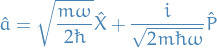
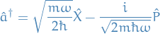
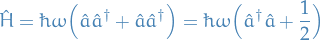
So we instead use the notation of
 and
and  which have the property
![\begin{equation*}
[ \hat{a}, \hat{a}^\dagger ] = 1
\end{equation*}](../../assets/latex/quantum_mechanics_437cd4aa86dd5274e5e835448fe308d9ced59efa.png)
Once again rewriting the Hamiltonian
Observe that
![\begin{equation*}
[ \hat{H}, \hat{a} ] = - \hbar \omega \ \hat{a}
\end{equation*}](../../assets/latex/quantum_mechanics_c327ba7d4fd17a0a95440c738d7aa8b70d19d63b.png)
Conider the following operation:
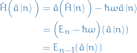
where we in the last line used the fact that for a simple Harmonic Oscillator
 .
.
Thus,

I.e. applying
to an eigenfunction gives us the eigenfunction of the  eigenstate.
We call this operator the annhiliation or lowering operator.
We can do exactly the same of
to observe that

which is why we call
the creation or rising operator.
Buuut there's a problem: we can potential "annihilate" below to a state with energy below zero! To fix this we simply define the ground state such that

Thus,
And all other higher energy states can then be constructed from this, by successsive application of
- Normalizing the lowering- and raising-operator

Thus,

Doing the same for
, we get

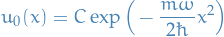
- Solving for the ground-state
We can find the proper solution for the ground-state by solving the differential equation

And substituting in for
both the and  , so that we get the differential equation. Solving this, we get
- Normalizing the lowering- and raising-operator
Solving the differential equation
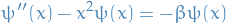
We start of by rewriting the Schrödinger equation for the harmonic oscillator:
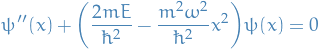
Letting , we have
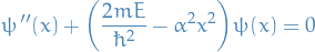
We'll require our solution to be normalizable, i.e. square-integrable, therefore we need the differential equation to be satisfied as  , in which case we can drop the constant term:
Letting  which is just a constant (apparently…), we have
I'm not sure I'm "cool" with this. There's clearly something weird going on here, since  is a parameter of the potential, NOT a variable which we can just set.
Letting  , we then have
Therefore we instead consider the simpler problem:
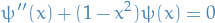
where we've dropped the  , which we will include later on through the us of method of variation of parameters. This clearly has the solution

Now, using method of variation of parameters, we suppose there exists some particular solution of the form:

For which we have
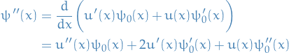
Substituting into the diff. eqn. involving ,

Since  satisfies the original equation, we have

Seeing this, we substitute in our solution for  ,
,

Thus,

Which, if we let

gives us

which we recognize as Hermite differential equation! Hence, we have the solutions
Why the though? Well, if you attempt to solve the Hermite equation above using a series solution, i.e. assuming
you end up seeing that you'll have a recurrence relation which depends on the integer , and further that for this to be square-integrable we require the series to terminate for some , hence you get that dough above.
Also, it shows us that we do indeed have a (countably) infinite number of solutions, as we'd expect from a Sturm-Liouville problem such as the Schrödinger equation :)
Correspondance principle
The correspondence principle states that the behavior of systems described by quantum mechanics reproduces the classical physics in the limit of large numbers.
Operators
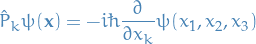
Momentum

"Derivation"
Considering the wave equation of a free particle, we have
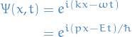
Taking the derivative of the above, and rearranging, we obtain:
![\begin{equation*}
p \big[ \Psi(x, t) \big] = - i \hbar \frac{\partial}{\partial x} \big[ \Psi(x, t) \big]
\end{equation*}](../../assets/latex/quantum_mechanics_e9d4453e606f945090485ae9d0290df6002f09da.png)
and thus we have the momentum operator

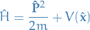
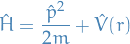
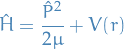
Hamiltonian
"Derivation"
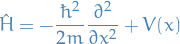
Where the Hamiltonian comes from the fact that for TISE we have the following:
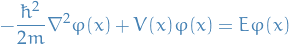
which we can then write as:
![\begin{equation*}
\Big[ - \frac{\hbar^2}{2m} \nabla^2 + V(x) \Big] \varphi(x) = E \varphi(x)
\end{equation*}](../../assets/latex/quantum_mechanics_8bb0ba994b3bb23184cb1145a8f97a41fbf95342.png)
and we have our operator  !
!
In the above "derivation" of the Hamiltonian, we assume TISE for convenience. It works equally well with the time-dependence, which is why we can write the TIDE expression using the Hamiltonian.
In fact, one can deduce it from writing the wave-function as a function of  and , and then note the operator defined for the momentum . This operator can then be substituted into the classical formula for the energy to provide use with a definition of the Hamiltonian operator.
Theorems
Conserved operators
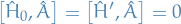
A time-independent operator is conserved if and only if ![$[\hat{H}, \hat{O}] = 0$](../../assets/latex/quantum_mechanics_0e8e7c400c52fc780f5169d1701b8510b3d8e98a.png) , i.e. it commutes with the Hermitian operator.
, i.e. it commutes with the Hermitian operator.
Coherence
Stack excange answer
This guy provides a very nice explanation of quantum coherence and entanglement.
Basically what he's saying is that coherence refers to the case where the wave-functions which are superimposed to create the wave-function of the particle under consideration have a definite phase difference , i.e. the phase-difference between the "eigenstates" is does not change wrt. time and is not random .
Another answer to the same question says:
"It is better to think of there being one and only one wavefunction that describes all the particles in the universe."
Which is trying to make sense of entanglement, saying that we can look at the "joint probability" of e.g. two particles and based on measurement taken from one particle we can make a better judgement of the probability-distribution of the measurement of the other particle. At least this is how I interpret it.
Observables
Each dynamic variable is associated with a linear operator, say  , and it's expectation can be computed:
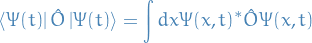
when there is no ambiguity about the state in which the average is computed, we shall write

The possible outcomes of an observable is given by the eigenvalue of the corresponding operator , i.e. the solutions of the eigenvalue equation:

where  is the eigenstate corresponding to the eigenvalue
  .
.
Observables as Hermitian operators
Observables are required to be Hermition operators, i.e. operators such that for the operator

where  is called the Hermitian conjugate of .
We an operator corresponding to an Observable to be a Hermitian operator as this is the only way to ensure that all the eigenvalues of the corresponding operator are real, and we want our measurements to be real, of course.
Compatilibity Theorem
Given two observables  and
and  , represented by the Herimitian operators
  and
and  , then the following statements are equivalent:
- and are compatible
- and have a common eigenbasis
- and commute, i.e.:
![$[\hat{A}, \hat{B}] = 0$](../../assets/latex/quantum_mechanics_81fb46d729367fa031cd2235cf831733ac641fb3.png)
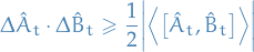
Generalised Uncertainty Relation
If  and
and  denote the uncertainties in observables
  and
and  respectively in the state
  , then the generalised uncertainty relation states that
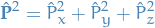
Momentum
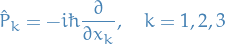
Then
And we have commutability, and thus the we can interchange the order of derivation
![\begin{equation*}
[ \hat{P}_k, \hat{P}_l ] = 0 \quad \iff \quad \frac{\partial^2}{\partial x_k \partial x_l} \psi(\mathbf{x}) = \frac{\partial^2}{\partial x_l \partial x_k} \psi(\mathbf{x})
\end{equation*}](../../assets/latex/quantum_mechanics_7658b0d23bc723beff7c1a5c272a23ed3ccbe578.png)
and
![\begin{equation*}
[\hat{X}_k, \hat{P}_l ] = i \hbar \delta_{k l}
\end{equation*}](../../assets/latex/quantum_mechanics_a027de200f6a6bd03149d7d3e73a77262e3bc648.png)
Hence,
where
Separation of variables
Here we consider the TISE for a isotropic harmonic oscillator in 3 dimensions, for which the potential is
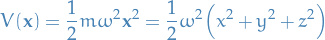
We can then factorize the Hamiltonian in the following way
Using this in the Schrödinger equation, we get

And we then assume that we can express  as
as

which gives us
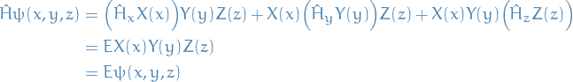
Which gives us
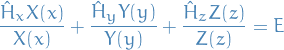
And since is a constant, we can write  , which gives us a system of equations
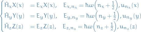
where  denotes the eigenfunction in the k-th dimension for the n-th quantised energy-level (remember we're working with a harmonic osicallator).
Which gives
denotes the eigenfunction in the k-th dimension for the n-th quantised energy-level (remember we're working with a harmonic osicallator).
Which gives

where  denotes the factors of the Hermite polynomials.
Angular momentum


Commutation
The interesting thing about the angular momentum operators, is that unlike the position- and momentum-operators in different dimensions does not commute!
![\begin{equation*}
[ \hat{L}_i, \hat{L}_j ] = i \hbar \ \varepsilon_{ijk} \hat{L}_k
\end{equation*}](../../assets/latex/quantum_mechanics_f8bde5f495abd6e1ba2602cd2d88deb66c4bf878.png)
This implies that the angular momentum in different dimensions are not compatible observables, i.e. we cannot observe one without affecting the distribution of measurements for the other!
Square of the angular momentum
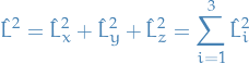
or in spherical coordinates,
![\begin{equation*}
\hat{L}^2 = - \hbar^2 \Bigg[ \frac{1}{\sin \theta} \frac{\partial}{\partial \theta} \Big( \sin \theta \frac{\partial}{\partial \theta} \Big) + \frac{1}{\sin^2 \theta} \frac{\partial^2}{\partial \phi^2} \Bigg]
\end{equation*}](../../assets/latex/quantum_mechanics_e278815117a1879fd90a7bb09ce03062e544f1c5.png)
We then observe that  is compatible with any of the Cartesian components of the angular momentum:
![\begin{equation*}
[\hat{L}^2, \hat{L}_x] = [\hat{L}^2, \hat{L}_y] = [\hat{L}^2, \hat{L}_z] = 0
\end{equation*}](../../assets/latex/quantum_mechanics_fe55448db26b86f1a2a21359463590e941836788.png)
which also tells us that they have a common eigenbasis / simultaneous eigenfunctions .
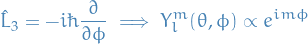
Angular momentum operators in spherical coordinates
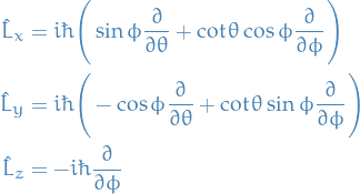
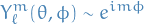
Eigenfunctions

where  and
and
![\begin{equation*}
Y_{\ell}^m (\theta, \phi) = (-1)^m \Bigg[ \frac{2 \ell + 1}{4 \pi} \frac{(\ell - m)!}{(\ell + m)!} \Bigg]^{-1/2} P_{\ell}^m ( \cos \theta ) e^{im \phi}
\end{equation*}](../../assets/latex/quantum_mechanics_6b0080c4bd12192170ef19bf5522f169365a378f.png)
with  known as the associated Legendre polynomials.
with known as the associated Legendre polynomials.
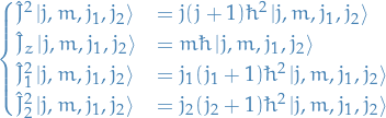
Quantisation of angular momentum
The eigenvalue function for the magnitude of the angular momentum tells us that the angular momentum is quantised. The square of the magnitude of the angular momentum can only assume one of the discrete set of values

and the z-component of the angular momentum can only assume one of the discrete set of values

for a given value of .
Laplacian operator

Angular momentum - reloaded
We move away from the notation of using  for angular momentum because what follows is true for any operator satisfying these properties.
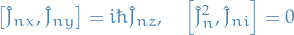
To generalize what the raising and lowering operators we found for the angular momentum we let 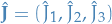 denote an (Hermitian) operator which satisfies the following commutation relations:
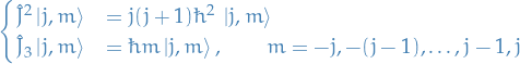
![\begin{equation*}
[\hat{J}_k, \hat{J}_\ell ] = i \hbar \varepsilon_{k \ell m} \hat{J}_m, \qquad \hat{J}^2 = \sum_{k} \hat{J}_k^2, \qquad [ \hat{J}^2, \hat{J}_k ] = 0
\end{equation*}](../../assets/latex/quantum_mechanics_0d94e73b27f56d9bfa0d4ca74705817023e31037.png)
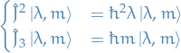
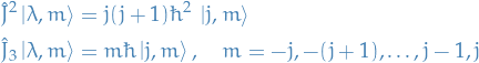
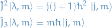
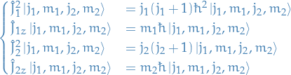
And since  and
and  are compatible, we know that these have a common eigenbasis, which we denote
  , and we write the eigenvalues in the following form:
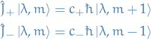
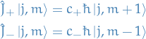
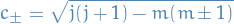
Further, we introduce the raising and lowering operators defined by:

for which we can compute the following properties:
![\begin{equation*}
[ \hat{J}^2, \hat{J}_\pm ] = 0
\end{equation*}](../../assets/latex/quantum_mechanics_114b4d8c8dc48f5d8a1bf1fe7d3a0b3e011ede3c.png)
![\begin{equation*}
[ \hat{J}_3, \hat{J}_\pm ] = \pm \hbar \hat{J}_{\pm}
\end{equation*}](../../assets/latex/quantum_mechanics_b83e24ac7ccf18b9fc35a2c0ee7b44e4a132c084.png)
I.e. we're working with a raising operator for  .
.
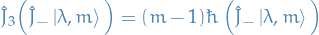
Considering the action of the commutator  on an eigenstate , we obtain the following:


which tells us that both  are also eigenstates of the but with eigenvalues
  , unless
  .
.
Thus  and
and  act as raising and lowering operators for the z-component of
  .
.
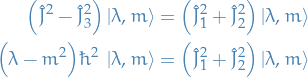
Further, notice that since  we have

Hence, the eigenstates generated by the action of  are still eigenstates of belonging to the same eigenvalue
  . Thus, we can write
where  are proportionality constants.
The notation used for the eigenstates 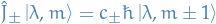 is simply saying that we know that the eigenvalue for does not change under the operator , and thus only the eigenvalue corresponding to
  changes with the factor
  (or rather another term of
  ) and so we denote this new eigenstate as
  .
.
To generalize the raising and lowering operators we found for the angular momentum we let denote an (Hermitian) operator which satisfies the following commutation relations:
And since and are compatible, we know that these have a common eigenbasis, which we denote  , and we write the eigenvalues in the following form:
with 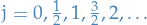
The set of  states
  is called a multiplet.
We introduce the raising and lowering operators defined by:
for which we can compute the following properties:
And we have the relations:
with

or, if we're assuming  , we have
There was originally also the relation

which I somehow picked up from the lecture. But I'm not entirely sure what this actually means…
Some proofs
Lowering operator on an eigenstate is another eigenstate

Where the RHS is due to the commutation relation we deduced earlier. This gives us the equation
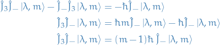
which tells us that is also an eigenstate of but with the eigenvalue  .
.
Just to make it completely obvious what we're saying, we can write the relation above as:
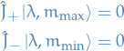
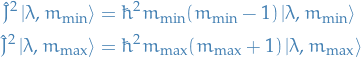
Eigenvalues are bounded
The eigenvalues of are bounded above and below, or more specifically

Further, we have the following properties:
Eigenvalues of
are  , where is one of the allowed values

 thus we label the eigenstates of and by rather than by
  , so that
- For an eigenstate
 , there are possible eigenvalues of
The set of states is called a multiplet
We start by observing the following:
Taking the scalar product with  yields

so that
Hence the spectrum of is bounded above and below, for a given . We can deduce that
Using the following relations:
and applying the to  and
and  in turn, we can obtain the following relations:

Using the notation  and using the equality above, we get the equation
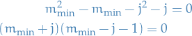
and we see that, since  by definition, the only acceptable root to the above quadratic is

Now, since  and
and  differ by some integer,
  , we can write

Or equivalently,

Hence, the allowed values are

for any given value of , we see that ranges over the values

which is a total of values.
Concluding the following:
Eigenvalues of
are , where is one of the allowed values
Since
we can equally well label the simultaneous eigenstates of and by rather than by , so that
- For a eigenvalue of , there are possible eigenvalues of , denoted by
 , where runs from to
- The set of states is called a multiplet
- Which step makes it so that the j in the case of "normal" angular momentum only takes on integer values?
In the case where we're working with "normal" angular momentum, the spherical harmonics are also eigenfunctions
 . Since we require that the wave function must be single-valued, the spherical coordinates must be periodic in
  with period
  :
:

this implies that
is an integer, hence must also be an integer.
Properties of J
 implies

I.e.
 , thus
  is positive definite
 such that

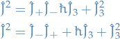
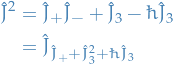
This is :
![\begin{equation*}
\begin{split}
\hat{J}_+ \hat{J}_- &= (\hat{J}_1 + i \hat{J}_2) (\hat{J}_1 - i \hat{J}_2) \\
&= \hat{J}_1^2 + \hat{J}_2^2 + i [\hat{J}_2, \hat{J}_1] \\
&= \hat{J}^2 - \hat{J}_3^2 + \hbar \hat{J}_3
\end{split}
\end{equation*}](../../assets/latex/quantum_mechanics_911ceee78d27d219e0244df53696cbbeaab6bfa0.png)
and
:
 ,
,  implies that
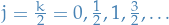
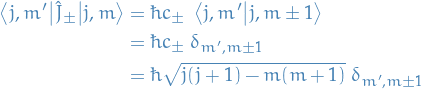
Normalization constant

![\begin{equation*}
\begin{split}
&= \bra{\lambda, m} \hat{J}^2 - \hat{J}_3^2 - \hbar \hat{J}_3 \ket{\lambda, m} \\
&= \hbar^2 [ j (j + 1) - m^2 - m ] \bra{\lambda m}\ket{\lambda, m} \\
&= \hbar^2 [ j (j + 1) - m^2 - m ] \\
\end{split}
\end{equation*}](../../assets/latex/quantum_mechanics_17e26b5174c4d5e56007613a2bab8d5de15ee763.png)
 we get

Computing the matrix elements

The matrix is 
And for the raising and lowering operators
Q & A
DONE Which step makes it so that the j in the case of "normal" angular momentum only takes on integer values?
In the case where we're working with "normal" angular momentum, the spherical harmonics are also eigenfunctions . Since we require that the wave function must be single-valued(?), the spherical coordinates must be periodic in with period :
this implies that is an integer, hence must also be an integer.
I'm not sure what they mean by "single-valued". From the notes they do this:
of which I'm not entirely sure what they mean.
From looking at looking at the spherical harmonics from a [BROKEN LINK: No match for fuzzy expression: *Spherical%20harmonics] the eigenvalue  for some non-negative integer
  , is due to regularity on the poles
  .
.
Central potential
Notation
 is the angle vertical to the xy-plane
- is the angle in the xy-plane
 is the mass (avoids confusion with the magnetic quantum number )
 is the position vector
 denotes the magnitude of the position vector
Stuff
![\begin{equation*}
\Bigg[ - \frac{\hbar^2}{2 \mu} \nabla^2 + V(r) \Bigg] u(\mathbf{r}) = E u(\mathbf{r})
\end{equation*}](../../assets/latex/quantum_mechanics_13bbbaed0b51bcbaa3c90d5ffd6342c6a32f24fc.png)
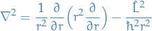
In spherical coordinates we write the Laplacian as

we can then rewrite this in terms of the angular momentum operator:
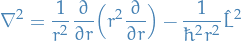
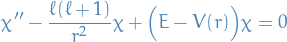
and thus the TISE becomes
![\begin{equation*}
\frac{h^2}{2 \mu} \Big[ - \frac{1}{r^2} \frac{\partial}{\partial r} \Big( r^2 \frac{\partial}{\partial r} \Big) + \frac{1}{\hbar^2 r^2} \hat{L}^2 \Big] u(r, \theta, \phi) = \big(E - V(r) \big) u(r, \theta, \phi)
\end{equation*}](../../assets/latex/quantum_mechanics_11e638756cc41efa66c97d677103f28bd6280626.png)
where  , then any pair of
  commutes, so there exists a set of simultaneous eigenstates
  .
.
Hydrogen atom
Notation
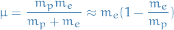
- effective mass of system


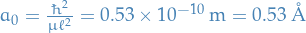
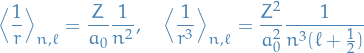
 is the Bohr radius

Stuff
Superposition of eigenstates of proton and electron
(Coloumb) potential:
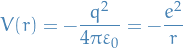
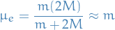
where the effective mass is
The TISE is:
![\begin{equation*}
\Big[ - \frac{\hbar^2}{2 \mu} \nabla^2 + V(r) \Big] \Psi(\mathbf{x}) = E \Psi(\mathbf{x})
\end{equation*}](../../assets/latex/quantum_mechanics_ed915b37098138dd5f7f255de76794f6f6c99b51.png)
We make the ansatz: 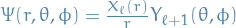
Thus,
Thus, we end up with
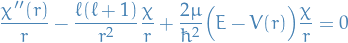
![\begin{equation*}
\Bigg[ \frac{\hbar^2}{2 \mu}\frac{d^2}{dr^2} - \frac{e^2}{r} + \frac{\hbar^2 \ell (\ell + 1)}{2 \mu r^2} \Bigg] \chi_{\ell}(r) = E \chi_{\ell} (r), \quad \chi_\ell(0) = 0
\end{equation*}](../../assets/latex/quantum_mechanics_5d7a57dcaaf7ea61855fd930d4fbea34b21a8e8c.png)
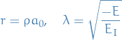
and we let
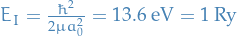
We now introduce some "scales" for length and energy:
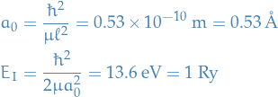
where  is the Bohr radius. Further, we let
Substituting these scales into the TISE deduced earlier:
![\begin{equation*}
\Bigg[ - \frac{\hbar^2}{2 \mu} \frac{1}{a_0^2} \frac{d^2}{d \rho^2} + \frac{\hbar^2 \ell (\ell + 1)}{2\mu a_0^2 \rho^2} - \frac{e^2}{a_0 \rho} - E \Bigg] \chi_{\ell}(a_0 \rho) = 0
\end{equation*}](../../assets/latex/quantum_mechanics_cb7a6f560631a5a4b60a73735b6382ba8d308cb2.png)
![\begin{equation*}
- E_I \Bigg[ - \frac{d^2}{d \rho^2} - \frac{\ell (\ell + 1)}{\rho^2} + \frac{2}{\rho} + \frac{E}{E_I} \Bigg] \chi_{\ell} (a_0 \rho) = 0
\end{equation*}](../../assets/latex/quantum_mechanics_eb52366033707e1f92bd3d6ea61d29457dbcfa19.png)
We tehn introduce another function of  instead of
  :
:

which gives us
![\begin{equation*}
\Bigg[ \frac{d^2}{d \rho^2} - \frac{\ell (\ell + 1)}{\rho^2} + \frac{2}{\rho} - \lambda^2 \Bigg] u_\ell(\rho) = 0
\label{tise-wrt-u-rho}
\end{equation*}](../../assets/latex/quantum_mechanics_17c59af110e339bfb23ad04579c83ea8ce5fe806.png) 1
1
with boundary conditions:  .
.
We then consider the boundary condition where  :
:
![\begin{equation*}
\rho \to \infty : \Bigg[ \frac{d^2}{d \rho^2} - \lambda^2 \Bigg] u_{\ell}(\rho) = 0 \implies u_{\ell}(\rho) = e^{\pm \rho \lambda}
\end{equation*}](../../assets/latex/quantum_mechanics_bc28652f07b4d56b79761bafdb60a859a5c65c49.png)
But since we need it to be bounded:

Another ansatz:  , which is simply the familiar method of variation of parameters, where we tack on another function of
  , the independent variable, to obtain another solution
  which is independent of
  .
.
If we then plug our  into the [tise-wrt-u-rho], which ends up being
![\begin{equation*}
y_{\ell}''(\rho) - 2 \lambda y_{\ell}' (\rho) + \Bigg[ - \frac{\ell (\ell + 1)}{\rho^2} + \frac{2}{\rho} \Bigg] y_{\ell}(\rho) = 0
\end{equation*}](../../assets/latex/quantum_mechanics_90918c8acb0edf8b06eb95c61ccc0a0429b23e16.png)
where due to the behaviour of  we have
Ansatz:
Spin - intrinsic angular momentum
Notation
 denotes the eigenstate of a system with spin (eigenvalue of
  )
)  in the z-direction, and being the eigenvalue of
 since the first number () is provided in the second anyways
 and
and 
 etc. we use to represent the coefficient of the function
  in some basis
- when we say a system has spin , we're talking about a system with eigenvalue of to be

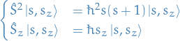
Stuff
Now that we know
![\begin{equation*}
[ \hat{J}_k , \hat{J}_l ] = i \hbar \varepsilon_{klm} \hat{J}_m
\end{equation*}](../../assets/latex/quantum_mechanics_3b516984539a54c7b52c023f4a3520ef48f77318.png)
- eigenvalues:
- eigenvalues:

From the orbital angular momentum, we have

In the case of orbital angular momentum , we have the requirement that  , which implies
  , rather than which we found in the Angular momentum - Reloaded.
 are diff. operators, which implies
  diff. operators
For a given value of ,  since
since  is the maximum for a spherical harmonic.

Now using the properties derived for the more general  operator we can deduce the all the other spherical harmonics by the usage of raising and lowering operators.
And it satisfies the commutation relation

and

Thus, we can construct a basis using the eigenstates of  , i.e. they form a C.S.O.C..
And as we've seen earlier, if an operator satisfies the above properties, we have:
- eigenvalues of :
 ,
, 
- eigenvalues of :

For a given value of ,  has
has  elements
And the eigenfunctions have the relations:
Example: system of spin 1 / 2
Since  , we have:
- eigenvalue of is

- eigenvalue of are

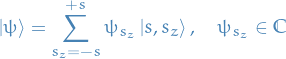
The basis of the space of the physical states is then
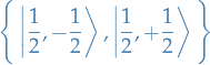
where we use the notation

Thus, any eigenstate we can expand in this basis:
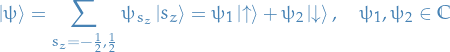
and then
 is the prob. of finding the system in
  measuring
 is the prob. of finding the system in
  measuring
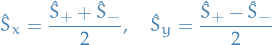
TODO Pauli matrices
Since we can write
Addition of angular momenta
Notation
 , without integer subscripts refers to the total angular momentum , and thus
  refers to the z-component of this total angular momentum
 refers to the z-component of the angular momentum indexed by, well, 1
 refers to the square of the angular momentum indexed by 1
Stuff
This excerpt from some book might be a really good way of getting a better feel of all of this
In this section we deal with the case of having two angular momenta!
For example, we might wish to consider an electron which has both an intrinsic spin and some orbital angular momentum, as in a real hydrogen atom.
Total angular momentum operator

where we assume  and
and  are independent angular momenta, meaning each satisfies the usual angular momentum commutation relations
where
 labels the individual angular momenta
 stands for cyclic permutations.
Furthermore, any component of  commutes with any component of
  :
:

so that the two angular momenta are compatible.
It follows that the four operators 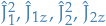 are mutually commuting and thus must posses a common eigenbasis!
This common eigenbasis is known as the uncoupled basis and is denoted  .
.
It has the following properties:
The allowed values of the total angular momentum quantum number , given two angular momenta corresponding to the quantum numbers  and
and  are:
are:

and for each of these values of , we have take on the values

The z-component of the total angular momentum operator commutes with and  , thus the set of four operators
 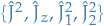 are also a mutually commuting set of operators with a common basis known as the coupled basis, denoted
  and satisfying
these are states of definite total angular momentum and definite z-component of total angular momentum but not in general states with definite or  .
.
In fact, these states are expressible as linear combinations of the states of the uncoupled basis, with coefficients known as Clebsch-Gordan coefficients.
I think what they mean by "states of definite angular momentum…" are the states which are coupled in a way that one eigenvalue decides the other?
TODO Example: two half-spin particles
Suppose we have two half-spin particles (e.g. electrons) with spin quantum numbers  and
and  .
.
According to the Addition theorem, the total spin quantum number takes on the values  and we require
  .
.
Thus, two electroncs can only have a total spin:
 called the triplet states, for which there are three possible values of the spin magnetic quantum number
 called the singlet states, for which there are only a single possible value
Let's denote the elements of the uncoupled basis as

where the subscripts 1 and 2 refer to electron 1 and 2, respectively. The operators  and
and  act only on the parts labelled 1, and so on.
If we let  be the state which has
  and
and  then it must have
  , i.e. total z-component of spin , and can therefore only be and not .
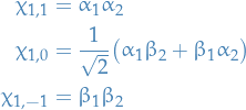
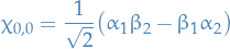
The eigenstates ends up being:
![\begin{equation*}
\begin{split}
\ket{s = 1, m_s = 1, s_1 = \frac{1}{2}, s_2 = \frac{1}{2}} &= \alpha_1 \alpha_2 \\
\ket{s = 1, m_s = - 1, s_1 = \frac{1}{2}, s_2 = \frac{1}{2}} &= \beta_1 \beta_2 \\
\ket{s = 1, m_s = 0, s_1 = \frac{1}{2}, s_2 = \frac{1}{2}} &= \frac{1}{\sqrt{2}} [ \alpha_1 \beta_2 + \beta_1 \alpha_2 ] \\
\ket{s = 0, m_s = 0, s_1 = \frac{1}{2}, s_2 = \frac{1}{2}} &= \frac{1}{\sqrt{2}} [ \alpha_1 \beta_2 - \beta_1 \alpha_2 ]
\end{split}
\end{equation*}](../../assets/latex/quantum_mechanics_fa572e88aaa427e9656062220ce71e930a158698.png)
Identical Particles
Stuff
Systems of identical particles with integer spin  known as bosons , have wave functions which are symmertic under interchange of any pair of particle labels (i.e. swapping the states of say two particles).
The wave function is said to obey Bose-Einstein statistics .
Systems of identical particles with half-odd-integer spins 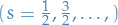 known as fermions , have wave functions which are antisymmetric under interchange of any pair of particle labels.
The wave function is said to obey Fermi-Dirac statistics .
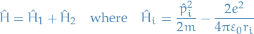
In the simplest model of the helium atom, the Hamiltonian is
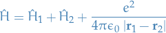
where
This is symmetric under permutation of the indices 1 and 2 which label the two electrons. Thus it must be the case if the two electrons are identical or industinguishable : it cannot matter which particle we label 1 and we which we label 2.
Due to symmerty condition, we have
Suppose that

so we conclude that  and
and  are both eigenfunctions belonging to the same eigenvalue . Further, any linear combination of the two is!
In particular, the normalised symmertic and antisymmertic combinations
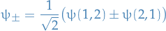
are eigenfunctions belonging to the eigenvalue .
If we introduce the particle interchange operator,  , with the property that

then the symmertic and antisymmertic combinations are eigenfunctions of with eigenvalues  respectively:

Since  are simultaneous eigenfunctions of
  and it follows that:

Fourier Transforms and Uncertainty Relations
This is heavily inspired by a post from mathpages.
Notation

 is such that
  , i.e. the ket corresponding to the eigenvalue
Stuff
Gaussian integral
- Basic
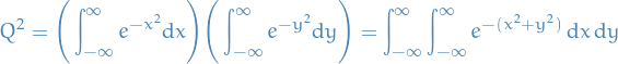
Taking the square of the integral
 we get
Reparametrizing in polar coordinates

which gives us the Jacobian transformation
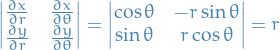
so the incremental area element is

Hence the double-integral above becomes
and we since
we get
Finally giving us

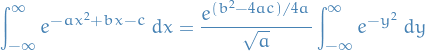
- More general
If we let
 , i.e. we consider some arbitrary quadratic, then
in terms of which we can write
Fourier transform of a normal probability density
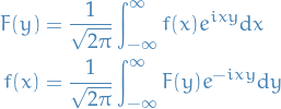
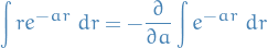
For any function  we have the relation
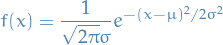
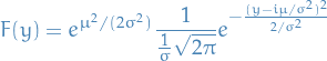
Now, if is a normal probability density, we have
which has the Fourier transform
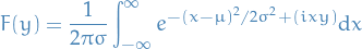
Where we can write the exponent in the integral of the form  with
with


hence the Fourier transform of the normal density function is
If we then choose our scales so that the mena of  is zero, i.e. so that
  the expression reduces to
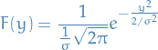
which means that the Fourier transform of a normal distribution with mean  and variance
  is a normal distribution with mean and variance
  .
.
Which tells us that the variances of the distributions and  satisfy the uncertainty relation:

This is the limiting case of the general inequality on the product of variances of Fourier transform pairs. In general, if is an arbitrary probability density and is its Fourier Transform, then
For any probability density function and it's the Fourier Transform  we have

and are two different ways of characterizing the same distribution, one in the amplitude domain and one in the frequency domain. Given either of these, the other is completely determined.
Remember, due to the Central Limit Theorem, i.i.d. the sample mean of any random variable with finite variance follows a Normal distribution
Hence, the equality above is saying that if we have an infinte number of realizations of some random variable  then the variance of this will be bounded below by the inverse of the variance of the Fourier Transform.
Hmm, I'm not 100% sure about all this. How can we for sure know that the Fourier Transform of the probability density will have a sample variance which decreases quicker than the actual density function ?
Why can we guarantee that the variance of the Fourier transform does not decrease faster than the variance of the density ?
We're saying that variance of random variable whos sample average converges to has a variance of  , which is fiiine. Then we're saying that some the variance of some random variable whos sample average converges to has a variance of
  , which is also fine. Then, we're saying that the variance of this random variable is always going to be greater than the limiting variances for these random variables, whiiiich you really can't say.
Application to Quantum mechanics
The canonical commutation relation is the fundamental relation between canonical conjugate quantities, i.e. quantities which are related by definition such that one is the Fourier transform of the other, which for two operators which are canonical conjugates, we have

Equivalently, if we have the above commutation relation between two Hermitian operators, then they form a Fourier Transform pair.
Where, if we take the commutation-relation the other way around the the sign of  changes, i.e. it's "symmetric" in a sense.
Now, if we then take some state  and compute the probability amplitudes that the measurements corresponding to the operators and will return the eigenvalues and
  respectively, then we find
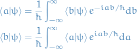
where  is the bra corresponding to the eigenstate with the eigenvalue of the operator .
That is; the probability amplitude distributions of two conjugate variables are simply the (suitably scaled) Fourier transforms of each other.
We saw earlier that the variances of two density distributions that comprise a Fourier transform pair satisfy the variance inequality:

Heisenberg Uncertainty Principle
How is this interesting? Well, as it turns out, the position operator  and the momentum operator
  have the commutation relation

which then tells us that they are conjugate varianbles, i.e. the probability amplitude distributions of the two are scaled Fourier transforms of each other! Which means they satisfy the following inequality

which is just the Heisenberg uncertainty principle!
Bra, kets, and matrices
Time-independent Perturbation Theory
Notation
 is the Hamiltonian corresponding to the unperturbed / exactly solvable system
 and represent the n-th eigenvalue and eigenfunction of the unperturbed Hamiltonian
 and
and  is the energy and ket of the i-th perturbation term
- and is the corrected (perturbed with all the terms) eigenvalue and eigenfunction, i.e.

 denote the total angular momentum (rather than a general ang. mom. as we've used it for earlier)
Overview
- Few problems in Quantum Theory can be solved exactly
- Helium atom: inter-electron electrostatic repulsion term in changes the problem into one which cannot be solved analytically
- Helium atom: inter-electron electrostatic repulsion term in
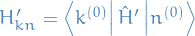
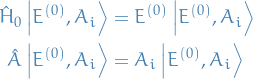
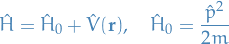
Perturbation Theory provides a method for finding approx. energy eigenvalues and eigenstates for a system whose Hamiltonian is of the form

where
is the Hamiltonian of an exactly solvable system, for which we know the eigenvalues, , and eigenstates,  , and
, and  is small, time-independent perturbation.
Does not converge
Perturbation does not actually guarantee convergence, i.e. that each term is smaller than the previous.
But, it is something called Borel summable, which is a method for summing up divergent series.
Short and sweet
Let

where:
- is a real parameter used for convenience
- is some small perturbation to the Hamiltonian, e.g.

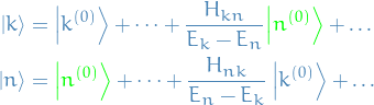
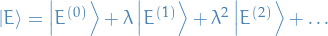
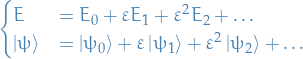
Then, the corrected eigenvalues and eigenfunctions are going to be given by:
"My" version (first order mainly)
It is convenient to consider the related problem of a system with Hamiltonian
where:
- is a real parameter used for convenience
- is some small perturbation to the Hamiltonian, e.g.
Then the eigenvalue problem we're trying to solve is then:
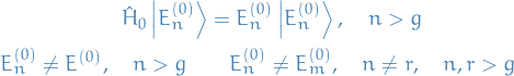
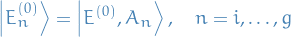
Assume and posses discrete, non-degenerate eigenvalues only, and we write:
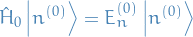
where are orthonormal.
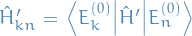
The effect of the perturbation on the eigenstates and eigenvalues is defined by the following maps:
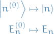
where
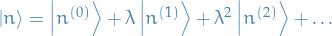
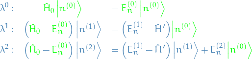
Thus, we solve the full eigenvalue problem by assuming we can exapnd and in a series as follows:
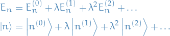
were the correction terms  and
and  are of succesively higher order of "smallness": the power of keeps track of this for us.
The correction terms are not normalized (by defualt)!
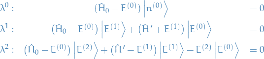
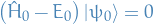
Substitute these into the equation for the full Hamiltonian (can be seen above):
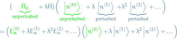
and equating the terms of the same degree of , giving:
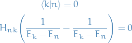
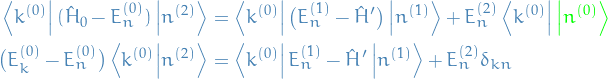
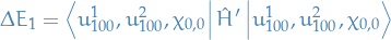
Now let's, for the heck of it, take the inner product of the coefficients of  with some arbitrary non-perturbed state
  :
:

which (due to being Hermitian), becomes

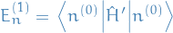
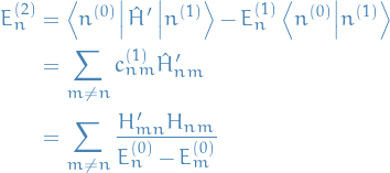
Let's first consider the correction (of first order) to the energy (then we'll to the eigenstate afterwards) by letting  (since is arbitrary):

LHS vanishes, and we're left with
which is the expression for the energy correction (of first order)!
To obtain the correction to the eigenfunction itself, we explore the following:  ,
,

where 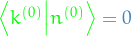 when , thus
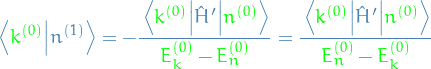
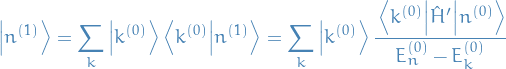
Hence, we can simply expand  in the basis of all :
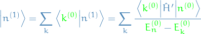
Aaaand we have our expression for the eigenstate correction (of first order)!
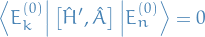
Preservation of orthogonality
Let's consider the inner product 
where we've picked out the terms which will be non-zero in . Observe that the non-zero terms are of different sign, thus
Thus orthogonality is preserved (for first order approximation).
Notes
Corrected
needs to be normalized, thus we better have

- We require that the level shift be small compared to the level spacing in the unperturbed system:
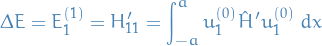
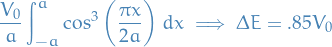
Example: Potential well

with
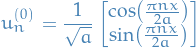
where  ,
,
Thus, the first order perturbation correction is
And the second order perturbation correction is
Letting , we have
Degeneracy in Perturbation Theory
Notation
- States are ordered s.t. first
 states are degenerate
Stuff
Remember, this is the case where has degenerate eigenstates, and we're assuming that the "real" Hamiltonian never is degenerate (which is sort of what you'd expect in nature, I guess).
Consider the eigenstate with degeneracy :

Then
We're just saying that we've ordered the states in such a way that we have state of degeneracy occuring in the first indices.
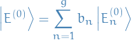
Since we have a g-dimensional subspace to work with for the degenerate eigenstate, now, instead of just finding the coefficients as in non-degenerate perturbation theory, we're looking for the "best" linear combination of the eigenbasis for the degenerate case!

and want to find the "optimal" coefficients / projection.
Proceeding as for the non-degenerate case, we assume that

where we assume we can write the following
Substituting the expansions into the eigenvalue equation and equating terms of the same degree , we find:
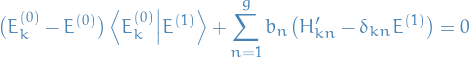
Once again, taking the scalar product with some arbitrary k-th unperturbed eigenstate  , we get

substituting in
we get
Now we consider the different cases of .
 - degenerate states
In this case we simply have  and thus the first term vanishes
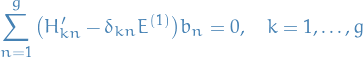
which is simply a "linear algebra eigenvalue problem" (when including for all )!
We'll denote the "linear algebra eigenvalues" as roots, to distinguish from the eigenvalues from the Schrödinger equation.

where

We get the roots  then have the different cases:
- distinct roots => we've broken the degeneracy of , yey!
- one or more repeating roots => there's still some degeneracy left from , aaargh!
- all equal roots => move on to 2nd order expansion, cuz 1st order didn't help mate!
If we have distinct roots, we end up with

Which is great; it's the same as the non-degenerate case! Therefore, we'd like to arrange for this to always be the case.
Suppose we can find some observable represented by an operator such that
Then there are simultaneous eigenstates of and :
If and only if the eigenvalues  are distinct, then we have a C.S.O.C., and we can write
Thus,
which is

Therefore,

Hence, if  for all
  , then is diagonal, as wanted.
Now, what if  are not distinct?! We then look for another operator , such that

i.e.  is a C.S.O.C., and letting
  we can repeat the about argument.
We're saying that if we can find some operator which commutes with both and , we can make diagonalizable, i.e. making our lives super-easy above.
 - non-degenerate states
We simply take our expansion for  and do exactly what we did for the non-degenerate case!
Example
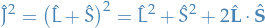
Central potential, spin-(1/2), spin-orbit interaction:
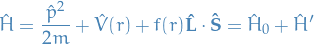
We know that

so if we use the coupled basis  , we can use the non-degeneracy theory to compute the 1st order energy shifts!
but

because of the  term in .
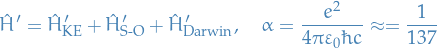
Example: Hydrogen fine structure
Notation
 denotes the spin-orbit term, whose physical origin is the interaction between the intrinstic magnetic dipole moment of the electron and the magnetic field due to the electron's orbital motion in the electric field of the nuclues
Stuff
with
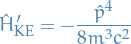
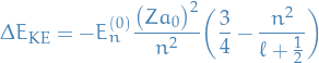
We start with the kinetic energy
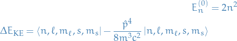
Where
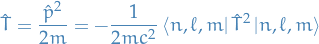
Therefore

Which appearantly give us
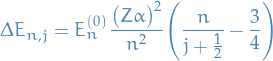
And for the spin-orbit interaction we have
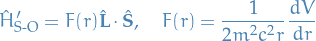
which gives us
Applying this to some ket

Thus,
where
thus, if
Which gives us
implying
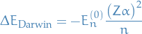
And finally for the Darwin-correction
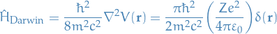
Observe that  as
as  for
for  , then

where
Which gives us the final Darwin correction
Giving the total correction
Example: Helium atom
Notation
 represents the spin-down state
 represents the spin-up state
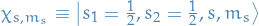 is the states for the coupled basis, where is the total spin quantum number and
  is the total magnetic quantum number
Neglecting mutual Coulomb repulsion between the electrons
Neglecting the mututal Coulomb repulsion between the electrons we end up with the Hamiltonian
It turns out that this yields the ground-state energy just

but experimentally we find

For the Helium atom we use the convention of denoting the ground state with  rather than
  as for the Hydrogen atom.
Stuff
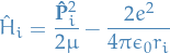
In the simplest model of the helium atom, the Hamiltonian is
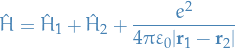
where
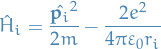
The term added to represents the repulsion of the two electrons, and in the  we have the negative term which represents the attraction.
Also, observe that this is symmertic under permutation of the indices which label the two electrons. Thus, the electrons are indistinguishable, as one would want.
The states of the coupled representation for the two spin-half electrons are the three triplet states:
and the singlet state:
- triplet states are symmetric under permutation
- singlet state is anti-symmetric under permutation
The overall 2-electron wavefunction is a product of a spatial wavefunction and a spin function:

The tensor product between the spatial wavefunction, , and the spin function,  , represents some function such that

where  is as defined above.
Thus, the total 2-electron wavefunction has the following symmetries:
symmetry of  |
symmetry of |
symmerty of  |
|
|---|---|---|---|
 (singlet) (singlet) |
anti | sym | anti |
 (triplet) (triplet) |
sym | anti | anti |
Consider the case of the Helium atom, where (if we're neglecting the inter-electron interactions) we would have the spatial solutions

since we can just use separation of variables and solve the Schrödinger eqn. for each electron separately, both having identical solutions.
Now, suppose further that , and thus  and
and  , then

Now consider the case where they would swap places, i.e. we were to interchange them (we're assuming they're completely opposite to each other, since i 2-electron orbit, they're almost always opposite of each other), then

Now, we know that

Therefore,  , as we have above, is symmetric:

Thus,

BUT we know that two fermions cannot occupy the same state at the same time, hence the above is not sufficient! We need the wave-functions to be different, further, for the wave-function of the entire Helium to stay the same we require the wave-functions to be anti-symmetric under interchanging of electrons (for  , that is). And this is why we introduce the described earlier
Ground state

Compute the first order correction to  , we compute the expectation of the perturbation , wrt. wavefunction:
which gives us a correction of

giving us the first order estimate of the ground-state energy

which is pretty close to the experimentally observed value of  .
.
Stuff
Define a new operator

With

Then we want to expand wrt. 
Setting up the Schrödinger equation, we have

Now, collecting terms involving the different factors of , we have:
For
 we find:
and therefore
 has to be one of the unperturbed eigenfunctions
  and
and  , i.e. the corresponding unperturbed eigenvalue.
For
 we have:
Which we can take the scalar product of with
:

Since
 , we have
Hence, the eigenvalue of the Hamitonian in this case becomes:
This is the correction to the n-th energy level! So to obtain the complete correction due to the perturbation, we have to do this for each of the eigenfunctions which make up the wave-function of the entire system we're looking at.
He atom


Time-dependent Perturbation Theory
Notation
- is the Hamiltonian corresponding to the unperturbed / exactly solvable system
- and represent the n-th eigenvalue and eigenfunction of the unperturbed Hamiltonian
- and is the energy and ket of the i-th perturbation term
- and is the corrected (perturbed with all the terms) eigenvalue and eigenfunction, i.e.


 is the density of final states
Expression for 
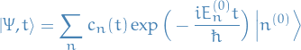
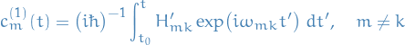
Solution to the TIDE can be written
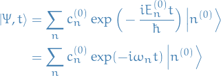
Generalize to the perturbed Hamiltonian

the coefficients
 become time-dependent:
Observe that lack of here!!!
We're not yet using the perturbation here, which would be
This is comes in the next section.
Probability of finding the system in the state
 at time
  is then
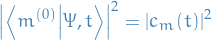
where we have used the orthonormality of
.
Substituting into TDSE:

which gives:
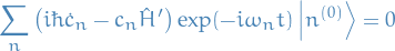
Taking scalar product with arbitrary unperturbed state
:

which gives:

Perturbation
Now consider the Hamiltonian related to the perturbed one above:

Assume we can expand
 in power series:

Substitute in the equation for
 derived above (factor of on RHS is from
  now instead of ):

Equate terms of same degree in
:
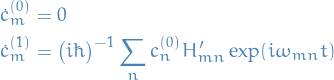
- Zeroth order is time-independent; since to this order the Hamiltonian is time-independent => recover unperturbed result
Integrating first-order correction gives:
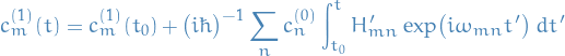
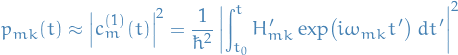
Suppose initially system is eigenstate of
, say , then for  , /probability of finding system in different state at time
Thus, transition probability of finding the system at a later time,
, in the state where  , is given by
TODO Time-independent pertubations for time-dependent wave equation
- Suppose is actually independent of time
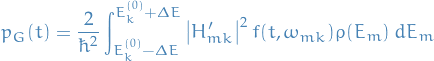
Fermi's Golden Rule
Interested in transitions not to single state, but to a group of final states,
 , in some range:

e.g. transitions to continuous part of energy-spectrum.
Total transition probability:
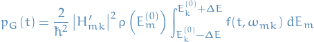
Assume
 to be small, s.t. can treat
  constant wrt.
  on this interval:
Change of variables
 , we get
where we've used
Number of transitions per time, the transition rate,  , is then just

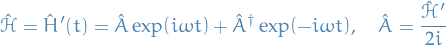
Harmonic Perturbations
Notation
 is the time-independent Hermitian operator
Stuff
- Transition probability amplitude is a sinusoidal function of itme which is turned on at time

Suppose that

where
is the time-independent Hermitian operator, which we write
Radiation
Notation
 is the dipole operator
Electromagnetic radiation
is the dipole operator where
- is unit charge
Einstein A-B coefficients
Notation
 is the absorption rate
 is the emission rate
 Einstein coeff. for spontanous emission
 Einstein coef. for stimulated emission
 dipole matrix elements
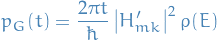
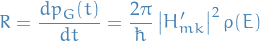
Spontanoues emission (thermodynamic argument)
We have
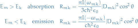
For absorption we have
![\begin{equation*}
\begin{split}
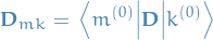
\dot{N}_{mk} &= N_k \rho(\omega_{mk}) B_{mk} \\
\dot{N}_{mk} &= R_{mk] N_k \\
B_{mk} &= \frac{R_{mk}}{\rho(\omega_{mk})} c \frac{R_{mk}}{I(\omega_{mk}}} \\
\implies B_{mk} & = \frac{\pi}{3 \hbar^2 \epsilon_0} |D_{mk}|^2
\end{split}
\end{equation*}](../../assets/latex/quantum_mechanics_a4141c89b669d5aacc3b6ecd2195364fb6559e66.png)
Now, suppose we have emission , with transition  :
:

Note that this is  , NOT as introduced earlier.
The distribution between the number of particles in the different states is then given by the Boltzmann distribution
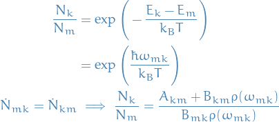
Plank's law tells us that Black body radiation follows
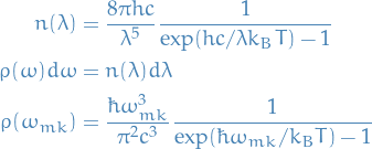
Which we can rewrite as

Substituting back into the epxression for spontaneous emission

One obtains the same result in QED.
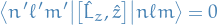
Selection rules
Goal is to evaluate .
Hydrogenic atom
- electric dipole operator is spin-independent
- work in uncoupled basis and ignore spin

Which implies
Which implies either of the following is true


This is called a selection rule.
Doing the same for  , we get

Considering the matrix elements, we get

which becomes

so we deduce that

giving the selection rule  .
.
We then conclude that the electric dipole transitions are only possible if

Which is due to
hence  would be zero unless
  .
.
Parity Selection Rule
- Under parity operator
 , electric dipole operator is odd multi-electron atoms
 - See notes :)
Quantum Scattering Theory
Notation
- is the scattering angle
- is the incident angle
 is the incident momentum
 is the scattering momentum (i.e. momentum after being scattered)
 , thus when we talk about the direction and so on of
  (wave-number), it's equivalent to the angle of the momentum
 is the solid angle
Rate of transitions from initial to final plane-wave states
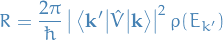
 is the density of the final states:
  is the number of final states with energy in the range
 denotes fixed potential (i.e. we say the "potential source" is fixed at some point and is then the position of the incident particle, and we treat the potential from the fixed scattering-particle as a regular "external" field)
Setup
- Beam of particles
- Each of momentum

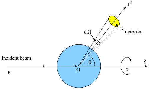
The incident flux is the number of incident particles crossing unit area perpendicular to the beam direcion per unit time.
The scattered flux is the number of scattered particles scattered into the element of solid angle about the direction , perunit time per unit solid angle.
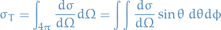
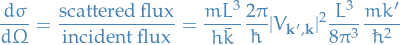
The differential cross-section is usually denoted  and is defined to be the ratio of the scattered flux to the incident flux:
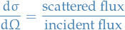
The differential cross-section thus has dimensions of area: ![$[L]^2$](../../assets/latex/quantum_mechanics_30b4b5cb961eecc96c323ceea58d701ae12b25ef.png)
Total cross-section is then
Born approximation
- Can use time-dependent perturbation teory theto approximate the cross-section
- Assume interaction between particle and scattering centre is localized to the region around

Hamiltonian
and treat
 as perturbation
- Wave-functions are non-normalizable, therefore we restrict to "potential-well" scenario, as we can take the width of the well as large as we "want"
- Since we're working in 3D: box-normalization
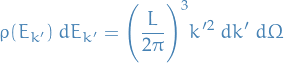
Density of final states
- Final-state vector
 is a point in k-space
 - All form a cubic lattice with lattice spacing
 (because of the potential well approx. discretizing the energy)
 - Volume of k'-sphere per lattice point is

# of states in volume element
 is
is
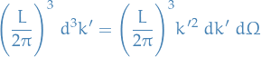
using spherical coordinates
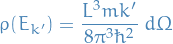
Energy is
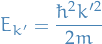
thus, the
, the density of states per unit energy, is the enrgy corresponding to wave-vector . Therefore,
is the # of states with energy in the desried interval and with
pointing into the solid angle about the direction  .
.
Final result for density of states
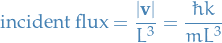
Incident flux
Box normalization corresponds to one particle per volume

Scattered flux
-
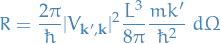
- Is # of particles scattered into per unit time
- Scattered flux therefore obtained by dividing by to get # of unit time per unit solid angle
Differential Cross-section for Elastic Scattering
Can compute the cross-section using scattered flux and incident flux found earlier
If potential is real, energy conservation implies elastic scattering, i.e.

The Born approximation to the differential cross-section then becomes
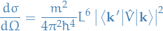
with

where  is called the wave-vector transfer.
(this is just the 3-dimensional Fourier transform of the potential energy function.)
Scattering by Central potentials
- Can simplify further
Work in polar coordinates
 , which refer to the wave-vector transfer so that

Then
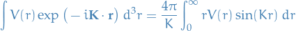
Born approximation then becomes
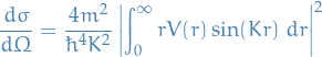
which is independent of
but depends on the scattering angle, , through  .
.
Trigonometry gives
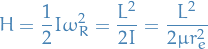
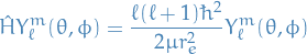
Quantum Rotator
- Two particles of mass
 and
and  separated by fixed distance
- Effective description of the rotational degrees of freedom of a diatomic molecule
- Choose centre-of-mass as origin: system is completely specified by angles and (since is fixed)
- Neglecting vibrational degrees of freedom, both
 and
and  are constant, and
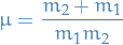
Since origin is frame of CM:
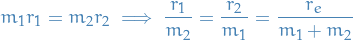
(Classically) Moment of intertia of the system is:
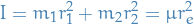
where
Classical mechanics:

where
 is the angular velocity of the system. The energy can be expressed as
Correspondance principle:

Since we're neglecting vibration,
is fixed, hence the wave function is independent of :
Two-body scattering
- So far assumed beam of particle scattered by fixed scattering centre; interaction described by
- Useful for electron-atom scattering due to regarding the atom as infinitively heavy
- Consider two-particle system; turns out it's the same!
Hamiltonian with relative separation
Centre of mass and relative position vectors
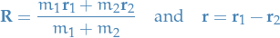
Then
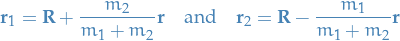
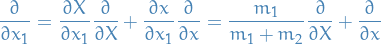
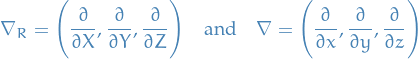
Rewrite gradient operators
 and
and  by
by
where
and so on.
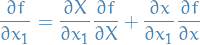
To see this just apply the differential operator wrt.  to some function :
Then
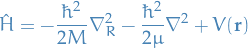
where
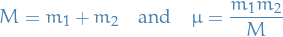
with
called the reduced mass
Can be viewed as
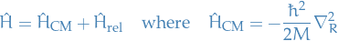
 describes free motation (kinetic energy) of centre of mass
In CM frame the CM is at rest, hence
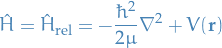
which is identical to the form of Hamiltonian of a single particle moving in the fixed potential
- Implies CM cross-section for two-body scattering obtained from solution to single particle of mass scattering from fixed potential
 Ion and Bonding
Notation
 is the mass of a proton
- is the mass of an electron
 reduced mass of the electron/two-proton system
 is the reduced mass of the two-proton system

- eigenfunction is called gerade if parity is even, and ungerade if the parity is odd
Stuff
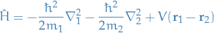
Schrödinger equation is
![\begin{equation*}
\Bigg[ - \frac{\hbar^2}{2 \mu_{12}} \nabla_R^2 - \frac{\hbar^2}{2 \mu_e} \nabla_r^2 - \frac{e^2}{(4 \pi \epsilon_0) r_1} - \frac{e^2 }{(4 \pi \epsilon) r_2} + \frac{e^2}{(4 \pi \epsilon_0) R} \Bigg] \psi(\mathbf{r}, \mathbf{R}) = E \psi(\mathbf{r}, \mathbf{R})
\end{equation*}](../../assets/latex/quantum_mechanics_844fc9792e787f53554a49a0ccbf6973c7a88b11.png)
- Nuclei massive compared to electrons, thus motion of nuclei much slower than electron
- Therefore, treat nuclear and electronic motions independently, further treat the nuclei as fixed, i.e. we only care about

Central Field Approximation
Notation
- is angular momentum quantum number
- is magnetic quantum number
- is mass
Stuff
Starting with the TISE, we have:
Rewriting in spherical coordinates, using the Laplacian in spherical coordinates and assuming

we have
![\begin{equation*}
\frac{\hbar^2}{2 \mu} \Bigg[ - \frac{1}{r^2} \frac{\partial}{\partial r} \bigg( r^2 \frac{\partial}{\partial r} \bigg) + \frac{1}{\hbar^2 r^2}\hat{L}^2 \Bigg] R(r) Y_{\ell}^m(\theta, \hpi) = \Big( E - V(r) \Big) R(r) Y_{\ell}^m(\theta, \phi)
\end{equation*}](../../assets/latex/quantum_mechanics_aff636d3c57d7a5a6ce07c5046ce69e4177d6a52.png)
which becomes:
![\begin{equation*}
\frac{1}{r^2} \frac{d}{dr} \Bigg( r^2 \frac{dR}{dr} \Bigg) - \frac{\ell (\ell + 1)}{r^2} R + \frac{2 \mu}{\hbar^2} \big[ E - V(r) \big] R = 0
\end{equation*}](../../assets/latex/quantum_mechanics_5ccf61ee8b9b365e46864854a5927d29ebb4f5e7.png)
Suppose

then the above equation becomes
Thus,
Substituting back into the equation we just arrived at, we obtain
Multiplying by
Which we can rewrite as

Therefore we consider this is a effective potential:
Example: charged nucleus
Consider the problem of an atom or ion containing a nucleus withcharge  and
and  elecrons.
We assume nucleus to be infinitively heavy and we assume only the following interactions are present:
- Coulomb interaction between each electron and the nucleus
- Mutual electronic repulsion
Then the Hamiltonian is
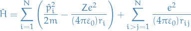
Presence of electron-electron interaction terms (2nd sum) means that the Schödinger equation is not separable.
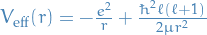
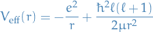
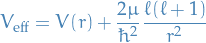
Therefore we introduce the Central Field Approximation, which is an example of a independent particle model , in which we assume that each electron moves in an effective potential  , which incorporates the nuclear attraction and the average effect of the repuslive interaction with the other
  electrons.
We expect this effective potential to have the following properties:
![\begin{equation*}
\lim_{r \to 0} V_{\text{eff}}(r) = - \frac{Ze^2}{(4 \pi \varepsilon_0) r} \quad \text{and} \quad \lim_{r \to \infty} V_{\text{eff}}(r) = - \frac{[Z - (N - 1)]^2 e^2}{(4 \pi \varepsilon_0) r}
\end{equation*}](../../assets/latex/quantum_mechanics_f794bd063ae01f789bbf88a2c1adf21aa00eca22.png)
 means the nucleus dominates
 means that we can treat (nuclues) + (the rest of the electrons) as a point-charge
Variational Method
- Especially useful for estimating the ground-state energy of a system
- This is closesly (if not "exactly") related to the Rayleigh quotient from Linear algebra
Main problem is guessing a trial function  :
:
- Recognize properties of the system and observe that ought to have the same properties (e.g. symmetry, etc.)
Useful identity:
Consider a system described by a Hamiltonian , with a complete orthonormal set of eigenstates  and corresponding energy eigenvalues
  ordered in increasing value

We observe that
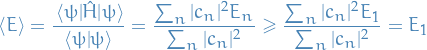
since  for all
  . Thus we have the inequality

Thus, we can estimate as follows:
- We chose a trial state
 which depends on one or more paramters
  .
. Calculate
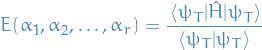
Minimize
 wrt. the variational parameters , by solving
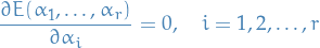
The resulting minimum value of  is then our best estimate for the ground-state energy of the given trial function.
Hidden Variables, EPR Paradox, Bell's Inequality
- Hidden variable theories suppose that there exist parameters which fully determine the values of the observables, and that QM is an incomplete theory where the wavefunction simply reflects the probability distribution wrt. to these parameters
EPR though experiment
- Two measuring devices (Alice and Bob)
- Electron sent from the middle where due to conservation of momentum (total spin needs to be conserved) we need:
- Alice to receive
 or
or 
- Bob receives the state which Alice does not
- Alice to receive
- Distance between measuring devices is too large to exchange any information between the the two measuring devices (even at speed of light)
Consider the following cases:
- Both measures spin-state in z-direction: measuring Alice's completely determines what we measures at Bob, due to spin being conserved
- Alice measures along z-direction, Bob measures along x-direction: measuring Alice's does not completely determine Bob's measure, rather, both spin-half states will be equally likely for Bob
The state of the "electron" measured by Bob will be correlated to the direction in which Alice makes the measurement!
Bell's Inequality
Notation
 spin component in direction
  of the particle travelling to , e.g.
  refers to taking on a specific configuration (remember we can only measure one of these directions)
 spin component in direction of the particle travelling to
  is the fraction of particle-pairs belong to the group
 denotes the probability of measuring
  and
and  together
Stuff
Since we're assuming that the spin-half pair is produced in a singlet state, this tells us immediately that

Suppose then that we're measuring  and
and  , we marginalize out all the other possible states to obtain the distribution:
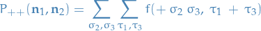
Observe that
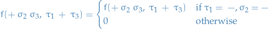
Thus,

Doing the same for the pairs  and
and  we observe that
The Bell's Inequality is for measurements made of two spin-half particles in directions  :
:

which defines a requirement which needs to be satisfied for a theory to be a realistic local theory.
Components possessing objective properties which exist independently of any mesaurements by observers and that the result of a measurement of a property at point cannot depend on an event at point sufficiently far from that information about the event at , even travelling at the speed of light, could not reach until after the measurement has taken place.
Theories meeting these requiremenets are called realistic local theories.
Quantum communication
Notation
 , i.e. these all denote the same thing
Convention to represent these two states

which is often parametrized in polar angles
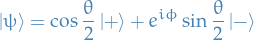
with
![$\theta \in [0, \pi]$](../../assets/latex/quantum_mechanics_5c3c0e9ea23efc5b0a5dbe637fa9ffdc48a38e69.png) and
and ![$\phi \in [0, 2 \pi]$](../../assets/latex/quantum_mechanics_79aa086b78e7b08c1293c05ca0ccc25029aeabc4.png) .
.
Bell's states:
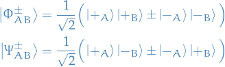
Secure communication
An entangled state between systems and implies the wavefunction of the combined and systems cannot be written as a tensor-product of independent wavefunctions for each system, i.e.

The Bloch sphere is just the parametrization of a two-qubit system in polar angles in 3d:
with and .
A frequently used complete set of two-qubit states in which both qubits are entangled, are the Bell states,
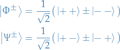
No-cloning theorem
It is impossible to create an identical copy of an arbitrary unknown quantum state.
Formally, let  where
where  denotes a Hilbert space.
Suppose we're in some initial state  , then initially we have

Then the question is: can we turn into a duplicate state of  ?
?
- Observing will collapse the state, thus corrupting the state we want to copy
- Can control of the system and evolve with unitary time evolution operator
 ,
where by unitary operator we mean that it preserves the norm and coherence.
,
where by unitary operator we mean that it preserves the norm and coherence.
Answer is no.
Suppose  on
on  such that
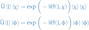
where and are two arbitrary states in .
 is the angle which in general can be a function of the states on which
  is acting. Then we have
![\begin{equation*}
\begin{split}
\bra{\chi}\ket{\psi} = \bra{\chi} \bra{j} \hat{U}^\dagger \hat{U} \ket{j} \ket{\psi} &= \exp \big[ i \big( - \Theta(j, \phi) + \Theta(j, \chi) \big) \big] \bra{\chi} \bra{\chi}\ket{\phi} \ket{\phi} \\
&= \exp \big[ i \big( - \Theta(j, \phi) + \Theta(j, \chi) \big) \big] \bra{\chi}\ket{\phi}^2
\end{split}
\end{equation*}](../../assets/latex/quantum_mechanics_457a20254f7bca6ad3b4988aef0e4bec70348d76.png)
This equation leads to the condition

I.e. states are either orthogonal or the same.
Quantum teleportation of a qubit
Two spin-half particles are prepared in the Bell state
![\begin{equation*}
\ket{\Psi_{AB}^-} = \frac{1}{\sqrt{2}} \Big[ \ket{+_A} \ket{-_B} - \ket{-_A} \ket{+_B} \Big]
\end{equation*}](../../assets/latex/quantum_mechanics_2407d9c5e7146a89e6175e268f43d42ee7d8079b.png)
- Establish a quantum channel by giving one of the electrons to Alice () and one to Bob (); due to the EPR-stuffs we know that if Alice makes a measurement, she can use a classicial channel to tell Bob which state she measured, which tells Bob that his electron is in the opposite state.
New particle given to Alice (Bob also knows that
 also takes this form)

Combine with the EPR states (referring to the ones Alice and Bob received beforehand)
![\begin{equation*}
\begin{split}
\ket{\Phi_{A' A B}} &= \frac{c}{\sqrt{2}} \ket{+_{A'}} \ket{\Psi_{AB}^-} + \frac{d}{\sqrt{2}} \ket{-_{A'}} \ket{\Psi_{AB}^-} \\
&= \frac{c}{2} \Big[ \ket{+_{A'}} \ket{+_A} \ket{-_B} - \ket{ +_{A'}} \ket{-_A} \ket{ +_B } \Big] \\
& \ + \frac{d}{2} \Big[ \ket{-_{A'}} \ket{+_{A}} \ket{-_B} - \ket{-_{A'}} \ket{-_A} \ket{+_B} \Big]
\end{split}
\end{equation*}](../../assets/latex/quantum_mechanics_27038b9c0ddef1cac90ff9f1c11285afa2d02f9f.png)
which we can rewrite in terms of the Bell-basis:
![\begin{equation*}
\begin{split}
\ket{\Phi_{A' A B}} =& \frac{1}{2} \Big[ \ket{\Psi_{A' A}^-} \big( - c \ket{ +_B} - d \ket{ -_B} \big) \\
& + \ket{\Psi_{A' A}^+ } \big( - c \ket{+_B} + d \ket{-_B} \big) \\
& + \ket{\Phi_{A' A}^-} \big( c \ket{-_B} + d \ket{+_B} \big) \\
& + \ket{\Phi_{A' A}^+} \big( c \ket{-_B} - d \ket{+_B} \big) \Big]
\end{split}
\end{equation*}](../../assets/latex/quantum_mechanics_9afc91f14d66f9c5aa646aaab2d542f917846982.png)
- Alice makes measurement of the two-state system consisting of and
 (this can in fact be performed physically)
- Collapses
 to one of the
  or
or 
- Alice now knows which of the states or her system is in
Breaks entanglement with
and forces to take on the "remainder" of the system, i.e. one of the

- Collapses
- Alice sends back to Bob which state
 collapsed to
- Since Bob knew the expression for
 , by learning which state
  is in, he can fully determine what state his own particle is in, i.e. the coefficient of
  and
and 
- This tells Bob which transformation he needs to perform to get his own particle into the state which was originally in!
- Since Bob knew the expression for
Superdense coding
Superdense coding is a procedure that utilises an entangled state between two participants in a way that one participant can transmit two bits of information through the act of sending over just one qubit.
Q & A
DONE Is there a correspondance between "unitary transformation / operator" and unitary matrices (when representing the operator as a matrix)?
Check out the definition of a
TODO Not quite sure about how representations used in the Superdense coding step-by-step procedure in the notes
Quantum computing
A quantum register is simply the entire state vector.
Usually we write it in the following form:
where:
 are called control or input register (does not necessarily make sense, it's just a term)
- are called the target or output register (does not necessarily make sense, it's just a term)
- and are states labelled by and bits
Example:  is a control ket specified by a binary number of length 2, i.e. a linear combination of the states
  ,
,  ,
,  , and
, and  .
.
Algorithms
Notation
 is called the oracle
Quantum register :
Deutch's algorithm
And we're wondering


 is working in
  , thus


where
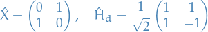
and

Applying the operator above, we get
![\begin{equation*}
\begin{split}
& \frac{1}{2 \sqrt{2}} \ket{0} \Big[ \ket{f_i(0)} - \ket{1 + f_i(0)} - \ket{f_i(1)} + \ket{1 + f_i(1)} \Big] \\
+ & \frac{1}{2 \sqrt{2}} \ket{1} \Big[ \ket{f_i(0)} - \ket{1 + f_i(0)} + \ket{f_i(1)} - \ket{1 + f_i(1)} \Big]
\end{split}
\end{equation*}](../../assets/latex/quantum_mechanics_abfa29fdca93df592b3e273419508009cf6eaa9b.png)
Thus, for  this leads to
![\begin{equation*}
\frac{1}{2} \ket{0} \Big[ \ket{f_i(0)} - \ket{1 + f_i(0)} \Big]
\end{equation*}](../../assets/latex/quantum_mechanics_e3b21c1942e1b7f3c2f5e40c6d382c1fd2bd1703.png)
and for  , we have
![\begin{equation*}
\frac{1}{2} \ket{1} \Big[ \ket{f_i(0)} - \ket{1 + f_i(0)} \Big]
\end{equation*}](../../assets/latex/quantum_mechanics_75da0a1b715f19feb0448aca6e065e4c22ab62a0.png)
i.e. just by looking at the control gate , we get the answer!
Grover's algorithm
- Search algorithm
- Reduces time-complexity to
 wrt. number of items
Cohen-Tannoudji - Quantum Mechanics
1. Waves and particles
Equations
Planck-Einstein relations
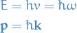
where is the wave vector s.t.  .
.
de Broglie
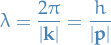
Eigenstates
With each eigenvalu is associated an eigenstate, i.e. an eigenfunction  s.t.
s.t.  where
where  is the time the measurement is performed, i.e. the measurement will always yield the same .
Scröding equation
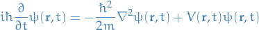
where  is the Laplacian operator
  .
.
- Free particle
No force acting on the particle →

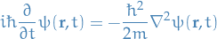
which has the solution

on the condition that
and satisty the relation:

According to de Broglie we have:

which is the same as in the classical case (no potential → only kinetic → get the above).
A plane wave of this type represents a particle whose probability of presence is uniform throughout all space :

- Form of the superposition
Principle of superposition tells us that every lin. comb. of plane waves satistfying the relation for
specified above, will also be a solution of the free-particle Schrödinger equation.
This super-position can be written:
![\begin{equation*}
\psi(\mathbf{r}, t) = \frac{1}{(2 \pi)^{3/2}} \int g(\mathbf{k}) e^{i [\mathbf{k} \cdot \mathbf{r} - \omega(\mathbf{k}) t]} d^3 k
\end{equation*}](../../assets/latex/quantum_mechanics_ae6f4147eda15fe7768be6390dc004fc547d3a36.png)
where
 represents the coefficients, and we integrate over all possible (
 ).
).
- Form of the superposition
- Time-independent potential
In the case of a time-independent potential,
 we have:
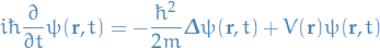
where
 is the Laplacian operator .
- Separation of variables. Stationary states
- Separation of variables
By making the assumption that
 can be separated as follows:

We can rearrange the Schrödinger equation as follows:
![\begin{equation*}
\frac{i \hbar}{\chi(t)} \frac{d \chi(t)}{dt} = \frac{1}{\varphi (\mathbf{r})} \Big[ - \frac{\hbar^2}{2m} \boldsymbol{\Delta} \varphi(\mathbf{r}) \Big] + V(\mathbf{r})
\end{equation*}](../../assets/latex/quantum_mechanics_f78ba49397ef630437a97e054fff0cea084e5cf0.png)
Where LHS only depends on
while RHS only depends on , which is only true if both sides are equal to a constant.
Setting LHS to
 (just treating as some arbitrary constant at this point), we obtain a solution for LHS:

Figure why we can set it to
.
Now do the same for RHS we get the final solution for the full plane wave function:

where we've let
 (which is fine as long as we incorporate the constant into
  ).
).
The time and space variables are said to be separated .
- Stationary States
The time-independent wave function makes it so that the Schrödinger Equation only involves a single angular frequency
. Thus, according to the Planck-Einstein relation, a stationary state is a state with a well-defined energy  (energy eigenstate).
We can therefore write the time-independent Schrödinger Equation as:
![\begin{equation*}
\Bigg[- \frac{\hbar^2}{2m} \boldsymbol{\Delta} + V( \mathbf{r} ) \Bigg] \varphi(\mathbf{r}) = E \varphi(\mathbf{r})
\end{equation*}](../../assets/latex/quantum_mechanics_9b07c50c656a0d2ed93a0d6759889fb3b646790b.png)
or:

where
is the differential operator :
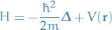
Which is a linear operator.
Thus
 tells us that applied to the "eigenfunction" (analogous to eigenvector) yields the same function, but multiplied by a constant "eigenvalue" .
The allowed energies are therefore the eigenvalues of the operator
.
I'm not sure about the remark by about the eigenvalues being the only allowed energies..
- Superposition of stationary states
We can then distinguish between the various possible values of the energy
(and the corresponding eigenfunctions ), by labeling them with an index :

and the stationary states of the particle have as wave functions:
And since
is a linear operator , we have a have series of other solutions of the form:
- Separation of variables
- Separation of variables. Stationary states
- Requirements
A system composed of only one particle → total probability of finding the particle anywhere in space, at time
, is equal to  :
:
We therefore require that the wave-function
must be square-integrable :
This is NOT true for the simplest solution to the Scröding equation:
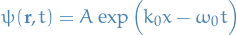
Where we have

And thus,
Hence it's NOT square-integrable.
They then say: "Therefore, rigorously, it cannot represent a physical state of the particle. On the other hand, a superposition of plane waves like [this one] can be square-integrable."
Heisenberg
- Deduction
Here we only consider the 1D case, allowing us to write the wave function as as superposition of over all possible
:
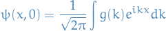
Suppose that
 has the following shape:

Now let
 be a function of s.t. :
Further, we assume that
varies sufficently smoothly within the interval ![$\Big[ k_0 - \frac{\Delta k}{2}, k_0 + \frac{\Delta k}{2} \Big]$](../../assets/latex/quantum_mechanics_0e943d3d48b06a789436f83cc1dd121bfa654e1b.png) . Then, when
. Then, when  is sufficiently small, we can approx. using it's tangent / linear approximation about the point
  :
:
![\begin{equation*}
\alpha(k) \simeq \alpha(k_0) + (k - k_0) \Big[ \frac{d \alpha}{d k} \Big]_{k = k_0}
\end{equation*}](../../assets/latex/quantum_mechanics_d991183de79508e6abb72ab5085133f80c3663e4.png)
which enables us to write the wave-function as:
![\begin{equation*}
\psi(x, 0) \simeq \frac{e^{i [k_0 x + \alpha(k_0)]}}{\sqrt{2 \pi}} \int_{-\infty}^{+\infty} |g(k)| e^{i(k - k_0)(x - x_0)} dk
\end{equation*}](../../assets/latex/quantum_mechanics_a2d7c405a98405c30a79084d18b650bf524a409e.png)
where
![\begin{equation*}
x_0 = - \Big[ \frac{d \alpha}{d k} \Big]_{k=k_0}
\end{equation*}](../../assets/latex/quantum_mechanics_7077a6149e94ccc5a218ec7faaae09483f8fafca.png)
I belive this note turned out to be that it was in fact integrating from
 to
to  .
.
I presume that when they write
 they mean "integrate from
  to
to  ..right? Since the "width" "contains" most of the integral.
This gives us a useful way of studying the variations of
 in terms of
  .
.
- If
 is large, i.e. is far from
  ,
,  will oscillate a very large number of times within the interval . Due to the high frequency the osciallations will cancel eachother out, thus
- If is small, i.e. is close to , will barely oscillate, and so we will end up with being a maximum.
- Relating to momentum
As seen previously,
 appears as a linear superposition of the momentum eigenfunctions in which the coefficient of
  is
is  . We are thus led to interpret
  (to within a constant factor) as the probability of finding
  if one measures, at
  , the momentum of a particle whose state is described by
  .
.
The possible values of
, like those of , form a continuous set, and is proportional to a probability density : the probability  of obtaining a value of between
  and
and  is, to within a constant factor
  . More precisely, we can rewrite the formula as:
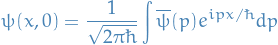
we know that
 and satisfy the Bessel-Parseval relation:
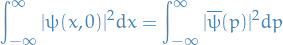
We then have
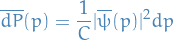
which is the probability that the measurement of the momentum will yield a result included between
and  .
.
Then, writing the relation
Honestly, I'm not seeing this.
This is based on the argument that
 for the
  to be significant, which I don't get.
- If
- Q & A
- DONE We're assuming a certain "family" of distribution for k; does this affect our deduction?
This
represents the coefficients for each of the different wave-functions ("different" meaning parametrized with different , and thus different wavelength / frequency), allowing us to write some arbitrary wave-function as a superposition of an infinite number of plane waves.
Why should it follow the "distribution" shown above? Why can't
have an arbitrary "distribution", e.g. multiple peaks?
- DONE What's up with the alphas on the boundary of the integrals?
- DONE Why is it the complex conjugate of the wave equation when writing it as a function of the momentum?
- DONE We're assuming a certain "family" of distribution for k; does this affect our deduction?
 .
.
Wave equation for free particle
Separable solution in as a function of and
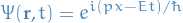
or
Complements
H: Stationary States of particle in one-dimensional square potential "well"
- Setup
Here we consider the time-independent Schrödinger Equation with a step-wise constant potential .
Thus, the time-independent Schrödinger Equation becomes:
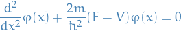
- Stationary wave-function in different potentials
We can solve the TISE with constant potential using integrating factors:
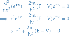
which we can be solved as a regular quadratic:
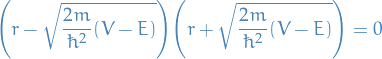
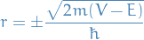
then whether or not we have a complex solution depends on whether or not
 is non-negative or not.
- E > V - energy of particle is GREATER than potential barrier
We write (
being defined by the the following equation)
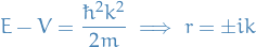
Then the stationary solution to the TISE with constant potential can be written

where
and are complex constants.
- E < V - energy of particle is LOWER than potential barrier
Let
be defined by the following equation
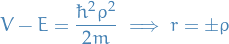
with solution to TISE with constant potential can be written:

where
and  are complex constants
Different order of
 and on LHS.
Also notice the fact that using the "integrating factor" to solve the ODE, our exponentials aren't positive in this case.
- E = V - energy of particle is equivalent to the potential barrier
In this case we simply end up with the differential equation
Which we can simply integrate twice and obtain a linear function expression for
 .
.
- E > V - energy of particle is GREATER than potential barrier
- Stationary wave-function at potential energy discontinuity
- Computation outline
- Solve the TISE with constant potential using integrating factors, leaving you with a quadratic.
- Let be such that
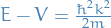 , for convenience
 - Obtain a general solution for both wave-functions depending on the
 in the different regions.
 - Assume the wave-function to be continues across the boundaries (discontinuities of the potential), i.e. we require
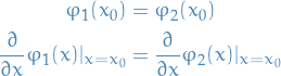
- Solve for the coefficients of the general solutions obtained.

In some cases, solving for all coefficients of the different wave-functions is not possible due to not having enough constraints.
In this case it might make sense to set some constant to zero, and instead solve for the ratios , not the coefficients themselves. Solving for ratios reduces the order of the system of equations by 1, and setting one of them to zero reduces it further by 1. In the case were we have a simple potential barrier in 1D, using the above methods to reduce the order then allows us to compute solve equations for the ratios, providing us with a reflection coefficient (which also implies a transmission coefficient ) and thus the probability of reflecting of the barrier.
- Potential well

We would follow the same as described above, but now we would have three wave functions, with boundary conditions:
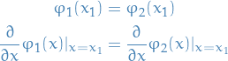
for the left side of the potential-well at
, and for the right side at  :
:
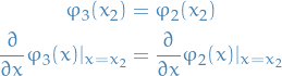
i.e. we simply use the exact same method, but now we have an additional boundary to consider.
The solution ends up looking as:
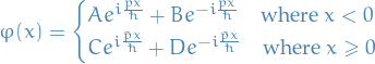
where we note that if we have a particle coming from the left, we set the coefficient of the left-traveling before the barrier to 0:

i.e. we can
We can "think" of each of these terms in the wave-function to be a super-position of eigenstates. Viewing it in that way, it makes a bit more sense I suppose.
- Infinite potential well
Same procedure as regular potential well, but now the wave-functions
 and
and  (i.e. wave-functions outside of the potential well) are equal to zero for all ! That is,

This leads us to the quantization of energies , where we have multiple solutions satisfying the boundary conditions specified above. If the potential well is of "width"
 , we end up with the solution
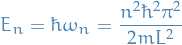
Which falls out of the fact that the boundary conditions above corresponds to the inverse wave-length being a integer multiple of the width of the potential well.
Each of these energy levels have their own eigen-function
 .
.
- Computation outline
2. The mathematical tools of quantum mechanics
Notation
 is the set of all square-integrable functions which are everywhere defined, continuous and infinitively differentiable. Together with the inner product
 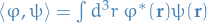 this defines a Hilbert space
 denotes a wave function
 is a ket or ket vector, which is an element or vector of
  space, e.g.
  is the state space of a particle, and is a subspace of a Hilbert space. It's defined such that we associate each square-integrable function
  with a ket vector, i.e.
 is the state space of a (spinless) particle in only one dimension
 is associated with a complex number, which is the scalar product, satisfying the properties of an inner product.
 denotes the set of linear functionals defined on the kets
  , which constitutes a vector space, called the dual space of .
 is a bra or bra vector of the space , which represents a linear functional
  , i.e. the linear function
  acting on the ket
  denotes a discrete basis
 denotes a continuous basis
 (
( ) denote a projection operator for a discrete (continuous) basis
 denotes the degeneracy of the eigenvalue
 denotes the i-th (degenerate) eigenvector corresponding to the eigenvalue , if this eigenvalue is non-degenerate then the
  in the super-script can be dropped
 denotes the eigensubspace of the eigenvalue of
Dirac notation
Overview
The quantum state of any physical system is characterized by a state vector, belonging to a space which is the state space of the system.
"Ket" vectors and "bra" vectors
- Dual space
A linear function
is a linear operation which associates an complex number with every ket :

Linear functional and linear operator must NOT be confused. In both cases we're dealing with linear operations, but the former associates each ket with a complex number, while the latter associates another ket.
- Generalized kets
"Generalized kets" are functions which are not necessarily square-integrable, but whose scalar product with every function of
 exists.
These cannot, strictly speaking, represent physical states. They are merely intermediaries.
The counter-examples to the "normal" definition of a ket are in the form of limiting cases, where the result of applying the bra to the ket is well-defined, but it's not square-integrable (it diverges when taking the limit) and thus not in
.
See the book at p.115 for more information about this.
But in short, in general, the dual space
and the state space are NOT isomorphic, except if is finite-dimensional.1 I.e. the following is true:
 2
2
But the otherway around is NOT true.
Linear operators
- Overview
Consider the operations defined by:

Choose an arbitrary ket
and consider:

We already know that
 ; consequently, the equation above is a ket, obtained by multiplying by the scalar
  . Therefore the
  applied to some arbitrary ket gives another ket, i.e. it's an operator.
If
 :
:
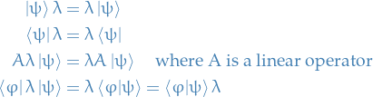
- Projections
Let
be a ket which is normalized to one:

Consider the operator
 defined by:

and apply it to an arbitrary ket
 :
:

Which is simply the projection of
onto : first take the inner product, not needing to normalize wrt. due  , and then multiply by to get the component.
We can also project onto a basis by taking the um over
 , and using this as an operator (applying each of them to the target ket as above). Thus we get the linear superposition .

 called the adjoint operator (or Hermitian conjugate ) of
Representations in state space
- Choosing a representation amounts to choosing an orthonormal basis, either discrete or continuous, in the state space
For a discrete basis
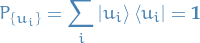
For a continuous basis
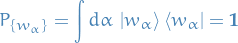
Representation of operators
Given a linear operator , we can, in a or basis, associate with it a series of numbers defined by

or for a continuous basis

We can then use the closure relation to compute the matrix which represents the operator  in the basis:
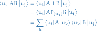
And equivalently for the continuous basis
Matrix representation of a ket
Problem: we know the components of and the matrix elements of the operator in some representation. How can we compute the components of  ?
?
In the basis, the "coordinate"  of
of  are given by:
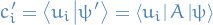
Inserting the closure relation between and , we obtain:
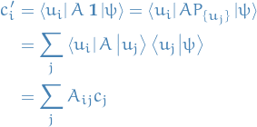
Or for a continuous basis we have:
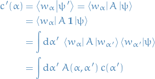
Eigenvalue equations for observables
is said to be an eigenvector (or eigenket ) of the linear operator if :

where . We call the equation above the eigenvalue equation of the linear operator .
We say the eigenvalue is nondegenerate if and only if the corresponding eigenvector is unique within a constant factor, i.e. when all associated eigenkets are collinear.
If there exists as least two linearly independent kets which are eigenvectors of with the same eigenvalue, this eigenvalue is said to be degenerate.
To be completely rigorous, one should solve the eigenvalue equation in the space , i.e. we ought to only consider those eigenvectors which have a finite norm.
Unfortunately, we will be obliged to use operatores for which eigenkets do not satisfy this condition. Therefore, we shall grant that vectors which are solutions of the eigenvalue equation can be
Two eigenvectors of a Herimition operator corresponding to two different eigenvalues are orthogonal.
Consider two eigenvectors and of the Hermitian operator .
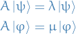
Since is Herimition, we can write the above using the corresponding bras:

Multiplying the above on the left with on the right:
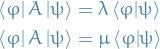
Which implies

Hence, if  we have orthogonality, i.e.
  .
.
The Hermitian operator is an observable if the orthonormal system of eigenvectors of , described by
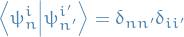
form a basis in the state space. That is,
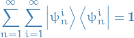
Sets of commuting observables
Consider an observable and a basis of composed of eigenvectors of .
If none of the eigenvalues of is degenerate, then the various basis vectors of can be labelled by the eigenvalue , and all the eigensubspaces are then one-dimensional. That is, there exists a unique basis of formed by the eigenvectors of . We then say that the observable constitutes, by itself, a C.S.C.O.
If, on the other hand, one or several eigenvalues of are degenerate, then the basis of eigenvectors of is not unqiue. We then choose another observable which commutes with , and construct an orthonormal basis of eigenvectors common to and . By definition, and form a C.S.C.O. if this basis is unique (to within a phase factor for each of the basis vectors), that is, if, to each of the possible pairs of eigenvalues  , there corresponds only one basis vector.
If we still don't have a C.S.C.O., we can introduce another Hermitian operator  which commutes with and , and then try to construct unique triples, and so on. This can be performed an arbitrary number of times in an attempt to obtain a C.S.C.O.
A set of observables  is called a complete set of commuting observables if
- All the observables commute by pairs
- Specifying the eigenvalues of all the operators determines aa unique (to within a multiplicative factor) common eigenvector
If  is a C.S.C.O., the specification of the eigenvalues
  determines a ket of the corresponding basis (to within a constant factor), which we sometimes denote by
Principles of Quantum Mechanics - Dirac
Notation
 denotes an eigenket belonging to the eigenvalue
  of the dynamical variable or a real linear operator
- If is an eigenvalue with multiple corresponding eigenkets, then
 denotes the ith corresponding eigenket
Definitions
Words
- conjugate complex
- refers to the complex conjugate of a number
- conjugate imaginary
- the bra
 corresponding to the ket
 - commutative operators

Linear Operators
Notation
 defines applying an operator to a bra
Theorems
Orthogonality theorem
Two eigenvectors of a real dynamical variable belonging to different eigenvalues are orthogonal .

Existence of eigenvectors / eigenvalues
- Simple case
Assume that the real linear operator
satisfies the algebraic equation:

which means that the linear operator
 produces the result zero when applied to any ket vector or to any bra vector.
Further, let the equation above be the simplest algebraic equation that
satisfies. Then
- The number of eigenvalues of is
- There are so many eigenkets of that any ket can be expressed as a sum of such eigenkets.
- The number of eigenvalues of
 be s.t.

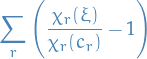
 in the above expression. In this case, each term of the sum above will be of the form:

 should vanish. I get the fact that
 Observables
Assumptions
If the dynamical system is in an eigenstate of a rea dynamical variable , belonging to the eigenvalue  , then a measurement of will certainly give as result the number . Conversely, if the system is in a state such that a measurement of a real dynamical variable is certain to give on particular result (instead of giving one or other of several possible results according to a probability law, as in the general case) then the state is an eigenstate of and the result of the measurement isthe eigenvalue of to which this eigenstate belongs.
I.e. we assume eigenstates to be the the case when a measurement of a real dynamical variable is certain to give one particular result.
Equations
Quantum Theory for Mathematicians
Notation
 represents the Hilbert space over
- Linear operator
 , with
  being the adjoint of
  denotes smooth functiosn on
  with compact support
2. A First Approach to Classical Mechanics
2.5 Poisson Brackets and Hamiltonian Mechanics
Let and be two smooth functions on  , where an element of is thought of as a pair
  , with
 representing position of a particle
 representing the momentum of a particle
Then the Poisson bracket of and , denoted  is the function on given by
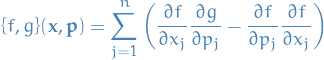
For all smooth functions , and  on we have the following:
 for all


Jacobi identity:

The position and momentum functions satisfy the following Poisson bracket relations:
If a particle in has the usual sort of energy function (kinetic energy plus potential energy), we have
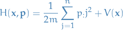
With the Hamiltonian, and as usual, having  , we can write Netwon's laws as:
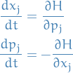
These equations we refer to has Hamilton's equations.
If  is a solution of the Hamilton's equation, then for any function on , we have
Call a smooth function on a conserved quantity if  is independent of for each solution of Hamilton's equations.
Then is a conserved quantity if and only if

In particular, the Hamiltonian is a conserved quantity.
Solving Hamilton's equatons on gives rise to a flow on , that is, a family  of diffeomorphisms of , where
  is equal to the solution at time of Hamilton's equations with initial conditions .
Since it is possible (depending on the choice of potential function  ) that a particle can escape to infinity in finite time, the maps are not necessarily defined on all of , but only on some subset therof.
If is defined on all of we say it's complete.
The flow associated with Hamilton's equations, for an arbitrary Hamitonian function , preserves the (2n)-dimensional volume measure

What this means, more precisely, is that if a measurable set is contained in the domain of for some  , then the volume of
  is equal to the volume of .
3. A First Approach to Quantum Mechanics
3.2 A Few Words About Operators and Their Adjoints
Linear operator
is bounded if

For any bounded operator
, there is a unique bounded operator , called the adjoint of , such that

- Existence of follows from the Riesz Theorem
For any bounded linear operator there is a unique bounded operator , called the adjoint of , such that
The existence of follows from Riesz Theorem.
We say is self-adjoint if  .
.
Further, if is a linear operator defined on all of  and having the property that

then is automatically bounded.
This means that an unbounded operator cannot be defined on the entire !
An unbounded operator on is a linear map from a dense subspace  into .
Then is "not necessarily bounded", since nothing in the definition prevents us from having  and having be bounded.
For an unbounded operator on , the adjoint of is defined as follows:
A vector  belongs to the domain
  of if the linear functional

defined on  , is bounded.
For  , let
, let  be the unique vector such that

Since  is bounded and is, by definition of a unbounded operator, dense, the BLT theorem tells us that has a unique bounded extension to all of .
Further, Riesz theorem then guarantees the existence and uniqueness of , the corresponding vector such that

Thus, the adjoint of a unbounded operator is a linear operator on .
An unbounded operator on is symmetric if

The operator is self-adjoint if

Finally, is essentially self-adjoint if the closure in  of the graph of is the graph of a self-adjoint operator.
3.6 Axioms of Quantum Mechanics: Operators and Measurements
The state of the system is represent by a unit vector in an appropriate Hilbert space .
If  and
and  are two unit vectors in with
  for some constant
  , then and represent the same physical state.
There is a more general notion of a "mixed state", which we will consider later.
To each real-valued function on the classical phase space there is associated a self-adjoint operator  on the quantum Hilbert space.
"Quantum Hilbert space" simply means "the Hilbert space associated with a given quantum system".
If a quantum system is in a state described by a unit vector  , the probability distribution for the measurement of some observable satisfies
![\begin{equation*}
\mathbb{E}[f^m] = \left\langle \psi, \big( \hat{f} \big)^m \psi \right\rangle
\end{equation*}](../../assets/latex/quantum_mechanics_8ff7f2646264c7f3bf12273db440e263ced746ad.png)
In particular, the expectation value for a measurement of is given by

Suppose a quantum system is initially in a state and that a measurement of an observable is performed.
If the result of the measurement is the number  , then immediately after the measurement, the system will be in a state
  that satisfies

The passage from to is called the collapse of the wave function. Here is the self-adjoint operator associated with by Axiom 2.
The time-evolution of the wave function in a quantum system is given by the Schödinger equtaion,
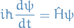
Here is the operator corresponding to the classical Hamiltonian by means of Axiom 2.
3.8 The Heisenberg Picture
In the Heisenberg picture, each self-adjoint operator evolves in time according to the operator-valued differential equation
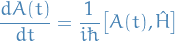
where is the Hamiltonian operator of the system, where  is the commutation, given by

4. The Free Schrödinger Equation
Notation

4.2 Solution as a convolution
"Free" means that there is no force acting on the particle, so that we may take the potential to be identically zero.
Thus, the free Scrhödinger equation is
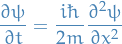
subject to an initial condition of the form

Suppose that is a "nice" function, for example, a Schwartz function.
Let  denote the Fourier transform of and define by
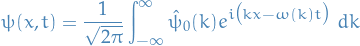
where  is defined by
Then solves the free Schödinger equation with initial condition  .
.
5. A Particle in a Square Well
6. Perspectives on the Spectral Theorem
Notation
- denotes the position operator given by

acting on

- is a self-adjoint operator
- Borel set of

 denotes the closed span of all eigenvectors of with eigenvalues in
- In cases where does not have true orthonormal basis, is called spectral subspace
- In cases where
 is the orthogonal projection onto
 For any unit vector
, we have

Indicator function
Goals of Spectral Theory
Recall that if the eigenvalues are distinct and
decomposes as
the probability of observing the value
 will be
  ., since
  is just the projection onto
  .
.
- In cases where does not have a true orthonormal basis of eigenvectors, we would like the spectral theorem to provide a family of projection operators
- One for each Borel subset

- Will allow us to define probabilities as in "standard" case above
- One for each Borel subset
- Call these projection operators spectral projects and the associated subspaces spectral subspaces.
- Intuitively, may be thought of as the closed span of all the generalized eigenvectors with eigenvalues in .
Position operator
- Has no true eigenvectors, i.e. no eigenvecors that are actually in
If we think that "generalized eigenvectors" for
are the distributions given by

then one might guess that spectral subspace
should consist of those functions that are "supported" on , i.e. a superposition of the "funtions"  with
with  should define a function supported on .
Spectral projection
is then orthogonal projection onto :

then
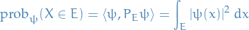
- The functional calculus of
- If
 then we should have
- If
7. Spectral Theorem for Bounded Self-Adjoint Operators
Notation
- is the separable complex Hilbert space
Operator norm of
on is
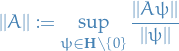
is finite.
- Banach space of bounded operators on , wrt. operator norm is denoted
 .
.  denotes the resolvent set of
  denotes the spectrum of
  denotes the projection-valued measure associated with the operator self-adjoint
 For any projection-vauled measure
and , we have an ordinary (positive) real-valued measure  given by

 is a map defined by
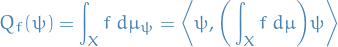
Spectral subspace for each Borel set

of
 defines a simultanouesly orthonormal basis for a family
  of separable Hilbert spaces
Properties of Bounded Operators
Linear operator
on is said to be bounded if the operator norm of
is finite.
Space of bounded operators on
forms a Banach space under the operator norm, and we have the inequality

for all bounded operators on
and .
For  , the resolvent set of , denoted is the set of all such that the operator
  has a bounded inverse.
The spectrum of , denoted by , is the complement in of the resolvent set.
For in the resolvent set of , the operator  is called the resolvent of at .
Alternatively, the resolvent set of can be described as the set of for which is one-to-one and onto.
For all , the following results hold.
- The spectrum of is closed, bounded and nonempty subset of .
- If
 , then is in the resolvent set of
Point 2 in proposition:hall13-quant-7.5 establishes that is bounded if is bounded.
Suppose satisfies  .
.
Then the operator  is invertible, with the inverse given by the following convergent series in :

For all , we have
![\begin{equation*}
\big[ \text{Range}(A) \big]^{\perp} = \text{ker}(A^*)
\end{equation*}](../../assets/latex/quantum_mechanics_041fde8f7e956e923e6e23df6a01ead0a29b2641.png)
Spectral Theorem for Bounded Self-Adjoint Operators
Given a bounded self-adjoint operator , we hope to associate with each Borel set  a closed subspace of , where we think intuitively that is the closed span of the generalized eigenvectors for with eigenvalues in .
We would expect the following properties of these subspaces:
 and
and 
- Captures idea that generalized eigenvectors should span
- Captures idea that generalized eigenvectors should span
- If and are disjoint, then

- Generalized eigenvectors ought to have some sort of orthogonality for distinct eigenvalues (even if not actually in )
- Generalized eigenvectors ought to have some sort of orthogonality for distinct eigenvalues (even if not actually in
- For any and ,

If
 are disjoint and
  , then
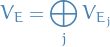
- For any , is invariant under .
If
![$E \subset [\lambda_0 - \varepsilon, \lambda_0 + \varepsilon]$](../../assets/latex/quantum_mechanics_bec5a95e47e8417fb8c1111121dd55490ad968ee.png) and
and  , then

Projection-Valued measures
For any closed subspace  , there exists a unique bounded operator
  such that
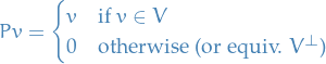
where  is the orthogonal complement.
This operator is called the orthogonal projection onto and it satisfies

i.e. it's self-adjoint.
One also has the properties

or equivalently,

Conversely, if is any bounded operator on satisfying  and
and  , then is the orthogonal projection onto a closed subspace , where

- Convenient ot describe closed subspaces of in terms of associated orthogonal projection operators
- Projection operator expresses the first four properties of the spectral subspaces; those properties are similar to those of a measures, so we use the term projection-valued measure
Let be a set and  an
an  in .
in .
A map  is called a projection-valued measure if the following properties are satisfied:
- For each
 ,
,  is an orthogonal projection
  and
and 
If
 are disjoint, then for all
  , we have
where the convergence of the sum is in the norm-topology on
.
- For all
 , we have
Properties 2 and 4 in of a projection-valued measure tells us that if and  are disjoint, then

from which it follows that the range of  and the range of
  are perpendicular.
Let be a in a set and let  be a projection-valued measure.
Then there exists a unique linear map, denoted
from the space of bounded, measurable, complex-valued functions on into with the property that
for all and all .
This integral has the following properties:
For all
, we have
In particular, the integral of the constant function
is  .
.
For all
, we have
Integration is multiplicative: For all
and , we have
For all
, we have
In particular, if
is real-valued, then  is self-adjoint.
By Property 1 and linearity, integration wrt. has the expected behavior on simple functions. It then follows from Property 2 that the integral of an arbitrary bounded measurable function can be comptued as follows:
- Take sequence
 of simple functions converging uniformly to
 - The integral of is then the limit, in the norm-topology, of the integral of the .
A quadratic form on a Hilbert space is a map  with the following properties:
 for all and
 the map
 defined by
![\begin{equation*}
\begin{split}
L(\phi, \psi) =& \frac{1}{2} \big[ Q(\phi + \psi) - Q(\phi) - Q(\psi) \big] \\
& - \frac{i}{2} \big[ Q(\phi + i \psi) - Q(\phi) - Q(i \psi) \big]
\end{split}
\end{equation*}](../../assets/latex/quantum_mechanics_6085b0f14f4edf2b5f0f23825c97cba9ce1cc8de.png)
is a sesquilinear form.
A quadratic form is bounded if there eixsts a constant such that

The smallest such constant is the norm of .
If is a bounded quadratic form on , there is a unique such that

If  belongs to for all , then the operator is self-adjoint.
Spectral Theorem for Bounded Self-Adjoint Operators: direct integral approach
Notation
- is a
 measure on a of sets in
 - For each
 we have a separable Hilbert space
  with inner product
- Elements of the direct integral are called sections
Stuff
There are several benefits to this approach compared to the simpler "multiplication operator" approach.
- The set and the function become canonical:
- The direct integral carries with it a notion of generalized eigenvectors / kets, since the space can be thought of as the space of generalized eigenvectors with eigenvalue .
- A simple way to classify self-adjoint operators up to unitary equivalence: two self-adjoint operators are unitarily equivalent if and only if their direct integral representations are equivalent in a natural sense.


Elements of the direct integral are called sections , which are functions on with values in the union of the , with property

We define the norm of a section by the formula
provided that the integral on the RHS is finite.
The inner product between two sections  and
and  (with finite norm) should then be given by the formula
Seems very much like the differential geometry section we know of.
- is the fibre at each point in the mfd.
- is the mfd.
First we slightly alter the concept of an orthonormal basis. We say a family  of vectors is an orthonormal basis for a Hilbert space if

and

This just menas that we allow some of the vectors in our basis to be zero.
We define a simultanouesly orthonormal basis for a family of separable Hilbert spaces to be a collection of sections with the property that

Provided that the function  is a measurable function from into
 ![$[0, \infty]$](../../assets/latex/quantum_mechanics_7c43cf12221cf82ea0f3550c49639ade5528d224.png) , it is possible to choose a /simultaneous orthonormal basis
, it is possible to choose a /simultaneous orthonormal basis  such that

is measurable for all and .
Choosing a simultaneous orthonormal basis with the property that the function

is a measurable function from into , we can define a section to be measurable if the function

is a measurable complex-valued function for each . This aslo means that the are also measurable sections.
We refer to such a choice of simultaneous orthonormal basis as a measurability structure on the collection .
Given two measurable sections and , the function
is also measurable.
Suppose the following structures are given:
- a measure space

- a collection
 of separable Hilbert spaces for which the dimension function is measurable
 - a measurability structure on
Then the direct integral of wrt. , denoted
is the space of equivalence classes of almost-everywhere-equal measurable sections for which
The inner product  of two sections and is given by the formula
8. Spectral Theorem for Bounded Self-Adjoint Operators: Proofs
Notation
- with spectral radius
Stage 1: Continuous Functional Calculus
Stage 2: An Operator-Valued Riesz Representation Theorem
Let be a compact metric space and let  denote the space of continuous, real-valued functions on .
Suppose  is a linear functioanl with the property that
  is non-negative if is non-negative.
Then there exists a unique (real-valued, positive) measure on the Borel sigma-algebra in for which
Observe that is a finite measure, with

where  is the constant function.
Practice problems
"Point-potential"
We have a potential of the form

which gives us the TISE:
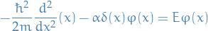
Then we impose the following conditions on the solution :
- continuity at
 , i.e. require
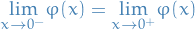
The continuity restriction does NOT necessarily mean that the derivative itself is continuous!
If we then integrate both sides of the TISE above over the interval  taking the limit
  :
:

which gives us

And since  , we get:
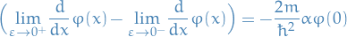
Then we compute the derivaties and take the limits, giving us something better to work with!
Harmonic Oscillator
Consider a potential energy of the form  . The classical energy is then:
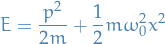
Using the Hamiltonian operator and the momentum  . We can then write the Schödinger equation, letting
  and
and  for convenience, as:
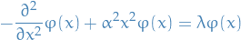
or equivalently,
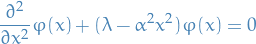
Goal is the to find solutions that are physical and suitable for all .
One approach is to perform the following:
- Obtain solution for limiting behavior
- Perform power series expansion
Our requirements for the solution:
- single valued over the region (well-behaved)
First consider when  is large and
  dominates with being negible by design . Then
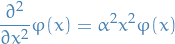
which we can guess ourselves to a solution of
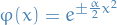
to which we then note that  is not satisfactory given that it diverges (due to restricting out attention to square-integrable functions only). Hence,
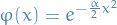
Why does it make sense to consider the limit behavior?
Due to the continuity imposed on the solution / wave function we now that the solution to the limiting behavior is related to the solution across the entire domain of .
From this solution we can then derive more solutions using reduction of order, i.e. we multiply our previous solution with some arbitrary function , which gives use
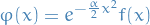
Taking the derivatives and substituting into the original differential equation we get:

To make the connection with a "special" function in a few steps, let's make the substituion  and replace the function with
  to get the following equation:
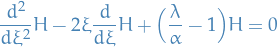
We can now represent as a power series:
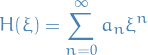
where we've made the assumption that this series converges for all and that the function is well defined.
Physically, we know the above has to be case for the solutions to make sense and satisfy our overall constraint that the integral of the probability density must be finite: 
Differentiating and substituting back into the differential equation we (eventually) obtain the recursion formula:
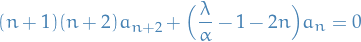
And thus we have a solution! BUT we have a serious problem :
- We assumed the series of to be convergent for all which is not generally true in the recursion relation for all values (the energy values) and
 (potential well curvature)
 - The function is square integrable if is truncated and does not contain an infininte number of terms in its series expansion
Thus, when we then require the
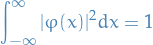
it can be seen from the recursion relation that the series expansion is finite (and hence converges  ) if
) if
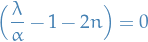
or the energy values have the folloiwgn discrete spectra,

Whiiiich we can finally write as:
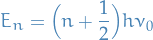
Short problems
Eigenvalue expansion of in angular momentum basis
The wavefunction of a particle at is known to have the form

where is an unknown function of .
What can be predicted about the results of measuring:
- the z-component of angular momentum?
- the square of the angular momentum?
Hint: expand  in eigenfunctions of
  , which are of the form
  , where
  .
.
Answer
Observe that
![\begin{equation*}
\cos 2 \phi = \frac{1}{2} \Big[ e^{2 i \phi} + e^{- 2 i \phi} \Big]
\end{equation*}](../../assets/latex/quantum_mechanics_dc5f97cf97be95cf2017b3107ff0423c7fa2fb50.png)
Thus,
![\begin{equation*}
u(r, \theta, \phi) = \frac{1}{2} A R(r) f(\theta) \Big[ e^{2 i \phi} + e^{- 2 i \phi} \Big]
\end{equation*}](../../assets/latex/quantum_mechanics_aba7987d568d0e5f2a195c6870511f2ac79511fc.png)
Thus, when measuring , we can obtain either  or
or  with equal probability.
We can't really say anything about , without knowing more about  , other than observing that
  since
since  .
.
Constructing matrix for angular component of a system with
Construct the  matrix which represent the Cartesian component in the z-direction of the angular momentum for a system with .
Answer
For ,  , and the matrix-elements of are given by
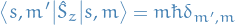
Thus, we have
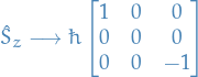
where we use  instead of
  to indicate that only corresponds to this matrix in this specific representation / space (Cartesian coordinates in this case).
Q & A
Simplification of potential well problem due to direction of travel
See rmk:potential-well-simplification-due-to-travelling-direction for what I'm talking about.
Footnotes:
Is is true that the Hilbert space  and its dual space are isomorphic; however, we have taken for the wave function space is a subspace of , which explains why
  is "larger" than .