Lagrangian Dynamics
Table of Contents
Notation
 position vector of particle of mass
 is velocity
 is linear momentum
 is kinetic energy
 is the unit vector perpendicular to
  (the unit position vector)
Stuff
Equations / Theorems
Galilean Transformation
Transforms from one inertial frame to another moving at constant velocity  relative to it

Then,

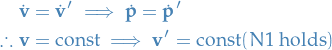
Conservation laws
Linear momentum
Angular momentum

Proof
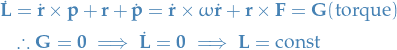
Remember, in this case we have  and thus $×
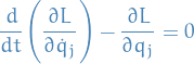
Lagrange's equations
Equations of motion in terms of generalised coordinates.
- equivalent to Newton's laws
- constraint equation have been eliminated
- constraint forces do not appear - they don't contribute to

Remember that the generalized forces are simply the forces projected onto the generalized coordinates  .
.
Derivation
We restrict our attention to functions of the form  , where
  denotes the generalised coordinates.
We assume Newton's Laws to be true in this derivation.
Since  we can apply the "cancellation of dots" which just says that for the case where
  is not a function of
  , then we have

thus,

Further,
![\begin{equation*}
\begin{align}
\frac{d}{dt} \Bigg[ \frac{\partial}{\partial \dot{q}_j} \Big(\frac{1}{2} m_i \dot{x}_i^2 \Big) \Bigg] &=
\frac{d}{dt} \big( m_i \dot{x}_i \big) \frac{\partial x_i}{\partial q_j} + m_i \dot{x}_i \frac{d}{dt} \Big( \frac{\partial x_i}{\partial q_j} \Big) \\
&= m_i \ddot{x}_i \frac{\partial x_i}{\partial q_j} + m_i \dot{x}_i \frac{\partial}{\partial q_j} \dot{x}_i \\
&= F_i \frac{\partial x_i}{\partial q_j} + \frac{\partial}{\partial q_j} \Big( \frac{1}{2} m_i \dot{x}_i^2 \Big) \quad & \text{by Newtons 2nd law}
\end{align}
\end{equation*}](../../assets/latex/lagrangian_dynamics_a0da3a3cb9c1ec46255e5eea377703e4e3d653e0.png)
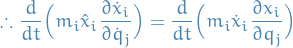
Summing over 
![\begin{equation*}
\frac{d}{dt} \Bigg[ \frac{\partial}{\partial \dot{q}_j} \Big( \sum_i \frac{1}{2} m_i \dot{x}_i^2 \Big) \Bigg]
\end{equation*}](../../assets/latex/lagrangian_dynamics_cf5376d9a657651bf7ef9bba0aece0889045511b.png)
we see that it's just the kinetic energy as a function of the generalised coordinates, velocities and time.
Thus,
![\begin{equation*}
\frac{d}{dt} \Bigg[ \frac{\partial}{\partial \dot{q}_j} \Big( \sum_i \frac{1}{2} m_i \dot{x}_i^2 \Big) \Bigg]
= \sum_i F_i \frac{\partial x_i}{\partial q_j} + \frac{\partial}{\partial q_j} \Big( \sum_i \frac{1}{2} m_i \dot{x}_i^2 \Big)
\end{equation*}](../../assets/latex/lagrangian_dynamics_6aba3617efaede628a055a04246aea0d6a3a578e.png)
where the first term is just  .
.
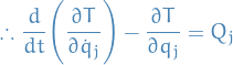
Since the constraint forces do now work, the sum over all constraint forces is zero.
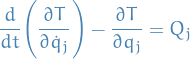
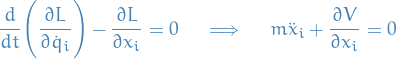
Therefore we end up with Lagrange Equations
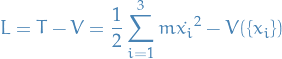
Using conservative forces
If the forces are conservative there exists a potential energy function such that
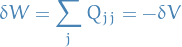
Assume $V = V(\{qj\}, t) then
Since  , we may write
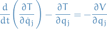
where 
This is for holonomic constraints.
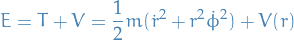
This applies to systems which also does not conserve their energy, unlike the usual

which is only valid for systems which conserve energy.
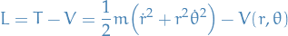
![\begin{equation*}
T = \frac{1}{2} m \Big[ \dot{r}^2 + (r \dot{\theta})^2 \Big]
\end{equation*}](../../assets/latex/lagrangian_dynamics_e75cd6b467160773dc5a7fa4cfcbbb4e6d3ddf11.png)


Definitions
Intertial frame
A frame in which Newtons 1st and 2nd laws hold.
Newtons Laws
Newtons 3rd law
Weak

for two objects  and
and  acting on each other.
Strong
Weak assumption AND  acts along
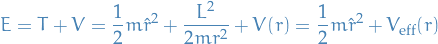
Effect potential
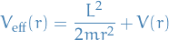
due to
where  gives us
Constraint force
Constraint forces do no work in any small instantaneous displacement of the system consistent with the constraints themselves.
Does not mea that the constraint forces can do no work during the actual motion of the system, e.g. a particle constrained to lie on a surface which is itself moving: there may then be a component of the actual particle velocity in the direction of the constraint force, so that work is done.
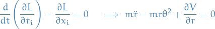
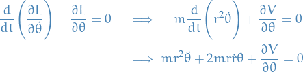
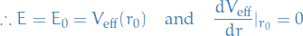
Circular orbits

Holonomic constraints
Example

i.e. it's a algebraic equation between the coordinates, not a differentiable relation and not an inequality.
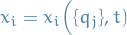
Generalised coordinates
Consider a system with  coordinates, i.e. 3D with
  particles each with coordinates, and let these coordinates be denoted by $xi,$ where
  .
.
That is, we're just "flattening" the  matrix to a vector.
If  holonomic constraints, not all
  are independent, and
  set of independent variables

We might have dependence between the due to the constraints being imposed, and thus representing the coordinates in the above way is just "removing" the dependence between the .
Hence, we end up with a basis of  dimensions.
Our aim is to derive  2nd order differential eq. for the set of generalised coordinates .
Transformation from  to
to  is invertible using constraint eq., that is:
 cannot be varied independently without violating the constraints, whereas we can vary while still satisfying the constraints.
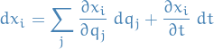
Generalised velocities
If denotes the generalised coordinates, then represents the generalised velocities.
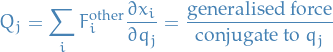
Generalised forces
Here  may have a component in the direction of a constraint force, due to motion, and so the constraint force may do work, e.q. a body on a surface is utself moving.
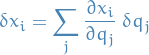
"Instantaneous", i.e. 
Then a small change consistent with constraints
In a virtual displacement the work done is
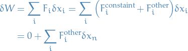
since constraint forces do no work.
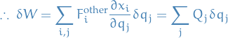
where