General Relativity
Table of Contents
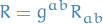
Notation
- IFs is inertial frames
Newtonian spacetime
Notation
Stuff
Reformulation of Poisson laws:

in terms of the Newtonian spacetime curvature as

where  is the 00-component of the Ricci tensor.
Then Newtonian spacetime is tuple  where
where
 is torsion free


Absolute space
Absolute space at time  is defined

and so (Newtonian) spacetime can be written as the disjoint union of the absolute spaces:

One way to visualize absolute time is as follows:

If absolute time didn't "flow uniformly", then we would allow something like the following, where we can have time standing completely still:

Motivation
Newton's laws
- Motion:
 and
and  where
where
 is the inertial mass
Gravity:
 where
where  , which satisfies the (gravitational) Poisson equation
where
 is Newton's gravitational constant
 is density
 is the mass of the "source"
Experiment: inertial mass is equivalent to gravitational mass, i.e.

which is called the weak equivalence principle, thus

Therefore we get the fact that locally, gravity is uniform acceleration
Non-uniform
 gives rise to tidal forces. Follows from the deviation equation
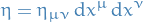
Special relativity
Spacetime
 where points are events, with inertial frames

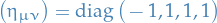
and we use the Minkowski metric
(a quadratic form), which is invariant in all IFs. Notice

- Motion is described by wordlines

- Free motion follow straight lines
- IFs related by Poincare group (which leaves
 invariant:
- Rotations
- Translations
- Lorentz boosts (rotation between space and time)
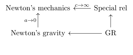
- Maxwell's eqns have Poincaré symmetry, but NOT Galilean symmetry (which is what Newton's gravity follows)
General relativity
- Laws of physics take same form in any coordinate system, i.e. invariant under general coord changes
- Will obtain by formuating laws with tensor fields
- There exists lcoal IF with no gravity, where laws are as in special relativity (called the /strong equivalence principle)
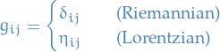
- Spacetime is (differentiable) manifold with Lorentzian metric
Postulates
Spacetime is a four-dimensional Lorentzian manifold  .
.
More specifically, (relativistic) spacetime is defined by the tuple  where
where
- is torsion-free
 is a Lorentzian metric
 is a time-orientation
Let  be a Lorentzian manifold.
Then a time-orientation is given by a smooth vector field that
- do not vanish anywhere, i.e.
 for all

Here  denotes an oriented atlas.
- Comparing with Newtonian spacetime we have gone from a "time"
 to a metric and time-orientation .
 - Reason for introducing a metric now is that we want some way of enforcing the fact that a particle cannot move faster than the speed of light
If we instead considered the metric
 then we observe that
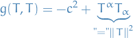
so if
, we are basically saying that the flow along has a "speed" which less than the speed of light (as we want).
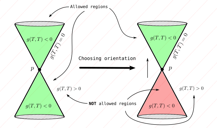
- Observe then that (with our convention), that
 is "illegal"
- Observe then that (with our convention), that
- The above produces the well-known light-cone, where if we make a choice of time-orientation to enforce the fact that a particle cannot move into the past
Connections and curvature
Notation
 denotes a basis of a vector fields on
  denotes the dual basis of covector fields on $M4
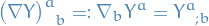
- In GR, the term connection will often be used to refer to the tensor ; this is because of how it relates to the connection 1-form
Covariant derivative as a (1, 1)-tensor field
with components
Components of connection

- Symmetric summation
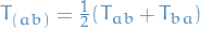 and anti-symmetric
 ![$T_{[ab]} = \frac{1}{2} (T_{ab} - T_{ba})$](../../assets/latex/general_relativity_9672d20ad207ab54cf472d1dfebc0705c67bcf77.png)
Torsion is denoted
 or in components
  and is given by

and in components
![\begin{equation*}
\tensor{T}{^{a}_{bc}} = - 2 \tensor{\Gamma}{^{a}_{[bc]}}
\end{equation*}](../../assets/latex/general_relativity_9ed0ab5cc30764f54c23a56993434cb5415e49b2.png)
Covariant derivative
Let be a basis of vector fields on . The components of the connection  in a basis is defined by

Letting

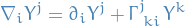
the covariant derivative can be written
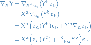
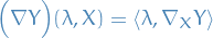
and so

where is the dual basis of . In a particular coordinate basis 
Under a basis change 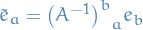 and
and 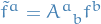 , we have

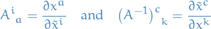
whre the basis change coefficients  .
.
In particular, under a change of coordinate basis, this becomes
![\begin{equation*}
\tensor{\tilde{\Gamma}}{^{i}_{jk}} = \pdv{\tilde{x}^i}{x^l} \pdv{x^m}{\tilde{x}^j} \pdv{x^n}{\tilde{x}^k} \tensor{\Gamma}{^{l}_{mn}} + \pdv{\tilde{x}^i}{x^l} \pdv[2]{x^l}{\tilde{x}^j}{\tilde{x}^k}
\end{equation*}](../../assets/latex/general_relativity_a63638edae388d7ae8284578c00d2d905f0dc3f3.png)
We use  to denote fixed indices, and
  for contractible ones.
![\begin{equation*}
\begin{split}
\tensor{\tilde{\Gamma}}{^{i}_{jk}} &= \left\langle \tilde{f}^i, \nabla_{\tilde{e}_k} \tilde{e}_j \right\rangle \\
&= \left\langle \tensor{A}{^{i}_{a}} f^a, \nabla_{\tensor{(A^{-1})}{^{c}_{k}} e_c} \tensor{\big( A^{-1} \big)}{^{b}_{j}} e_b \right\rangle \\
&= \tensor{A}{^{i}_{a}} \tensor{\big( A^{-1} \big)}{^{c}_{k}} \left\langle f^a, \nabla_c \tensor{\big( A^{-1} \big)}{^{b}_{j}} e_b \right\rangle \\
&= \tensor{A}{^{i}_{a}} \tensor{\big( A^{-1} \big)}{^{c}_{k}} \Big[ \tensor{\big( A^{-1} \big)}{^{b}_{j}} \underbrace{\left\langle f^a, \nabla_c e_b \right\rangle}_{=: \tensor{\Gamma}{^{a}_{bc}}} + \left\langle f^a , e_b \right\rangle e_c \Big( \tensor{\big( A^{-1} \big)}{^{b}_{j}} \Big)\Big] \\
&= \tensor{A}{^{i}_{a}} \tensor{\big( A^{-1} \big)}{^{c}_{k}} \tensor{\big( A^{-1} \big)}{^{b}_{j}} \tensor{\Gamma}{^{a}_{bc}} + \tensor{A}{^{i}_{a}} \tensor{\big( A^{-1} \big)}{^{c}_{k}} \tensor{\delta}{^{a}_{b}} e_c \Big( \tensor{\big( A^{-1} \big)}{^{b}_{j}} \Big) \\
&= \tensor{A}{^{i}_{a}} \tensor{\big( A^{-1} \big)}{^{c}_{k}} \tensor{\big( A^{-1} \big)}{^{b}_{j}} \tensor{\Gamma}{^{a}_{bc}} + \tensor{A}{^{i}_{a}} \tensor{\big( A^{-1} \big)}{^{c}_{k}} e_c \Big( \tensor{\big( A^{-1} \big)}{^{a}_{j}} \Big)
\end{split}
\end{equation*}](../../assets/latex/general_relativity_a21674ebe5974092b8b6308565c08007921dbdee.png)
If we then let  and
and  we obtain our proof (up to commutation between
  functions, so we're fine).
Moreover, in a specific chart  and changed basis
  we simply have
Substituting back into the above, we obtain our result.
Let be a connection on a smooth manifold .
A vector field  is said to be parallely transported along a curve with tangent vector field
  if
if

The parallel transport condition in components reads
Along an integral curve we have  , and so we can write
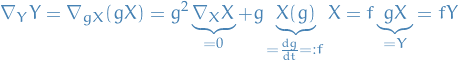
A geodesic is an integral curve of a vector field that satisfies

In other words, a geodesic vector field is parallely transported wrt. itself.
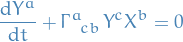
In a coordinate basis, the integral curves satisfy 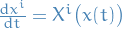 , and so the geodesic eqation is
![\begin{equation*}
\dv[2]{x^i}{t} + \tensor{\Gamma}{^{i}_{jk}} \Big( x(t) \Big) \dv{x^j}{t} \dv{x^k}{t} = 0
\end{equation*}](../../assets/latex/general_relativity_0fa018642bf1762d5f061424588acadcac57c584.png)
Consider a geodesic  with tangent field .
Suppose we reparametrize the curve so that  with
with  . The tangent field of the curve
  is then given by
  where
where  . Thus,
Thus, the equation  describes the same geodesic curve in a different parametrization.
An affine parameter is one for which  . We deduce that this means that
  for
for  and
and  .
.
Let  open for which
  is a bijection.
Normal coordinates at  , of a point
  , are given by
  where
where  are the components of

in a basis  .
.
In normal coordinates at 
Consider the geodesic through and  .
.
In normal coords. the geodesic takes the form

Inserting this into the geodesic equation and evaluating at  , we deduce that
Hence
Since this is true for all  in an open set
  , we have our proof.
Torsion and curvature
Torsion
Let be a smooth manifold with a connection .
The torsion is a  tensor defined by
where  are smooth vector fields.
One can easily check that this is indeed a tensor.
Componentwise,
![\begin{equation*}
\begin{split}
\tensor{T}{^{i}_{jk}} &= \left\langle f^i, T(e_j, e_k) \right\rangle \\
&= \left\langle f^i, \nabla_j e_k - \nabla_k e_j \right\rangle \\
&= \tensor{\Gamma}{^{i}_{kj}} - \tensor{\Gamma}{^{i}_{jk}} \\
&= - 2 \tensor{\Gamma}{^{i}_{[jk]}}
\end{split}
\end{equation*}](../../assets/latex/general_relativity_ad86c625dc2a571ccf7def5983fd145bb99605ba.png)
Geodesics are determined by the symmetric part of the connection components  , thus the torsion does not affect the geodesics!
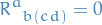
Let be a manifold with a connection .
For any function  ,
,

We prove this by working in a basis .
Since  , the covariant derivative of the covector
  is
is
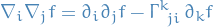
Therefore, antisymmetrising, we get
![\begin{equation*}
\nabla_i \nabla_j f - \nabla_j \nabla_i f = 2 \tensor{\Gamma}{^{k}_{[ij]}} \partial_k f = - \tensor{T}{^{k}_{ij}} \nabla_k f
\end{equation*}](../../assets/latex/general_relativity_728957436af238e8928074eb86b87f12047ceb69.png)
Since this is a relation between tensors, it follows that it must hold in any arbitrary basis.
Curvature
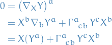
The Riemann curvature of a connection is a  defined by
![\begin{equation*}
R(X, Y) Z = \nabla_X \nabla_Y Z - \nabla_Y \nabla_X Z - \nabla_{[X, Y]} Z
\end{equation*}](../../assets/latex/general_relativity_46670b9c5172e188284c2939c36bc0253154e4b9.png)
where  are smooth vector fields.
One can verify that this is indeed a tensor by checking that it's linear in and  .
.
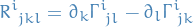
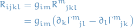
The Riemann tensor is the (1, 3) tensor defined by  , where the ordering of the arguments is standard notation. The components are then defined

The component-wise expression for the Riemann tensor can be seen as follows:
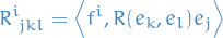
where we first observe that
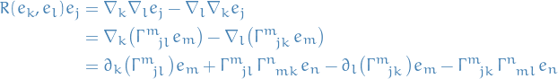
from which the Riemann tensor  immediately follows.
First, observe that for a torsionless connection , we have

Now
Since this holds for all , we conclude our proof.
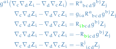
Let be a torsionless connection.
For any covector field 

Ricci identity (for vectors) says that for some vector field we have

We can write  , which gives us

We have

so

Locally

where we have dropped the resulting  terms since they commute in the lower indices.
Therefore
terms since they commute in the lower indices.
Therefore
Locally the coefficients of a covector field can be expressed as  for some vector field , so we simply let

and map indices  and
and  , giving us
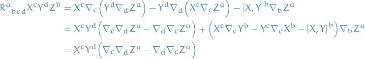
Riemann tensor has an important geometrical interpretation.
It can be shown that  is the change in upon parallel transport around a small quadrilateral whose opposite sides are integral curves of vector fields and . Hence, if
  parallel transport is locally path-independent.
The torsion and curvature of a connection vanish if and only if for any , there exists a chart such that  and
and

In short,

 tensor defined by contraction of the

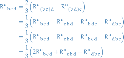
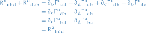
Suppose is a torsionless connection. Then we have
![\begin{equation*}
\begin{split}
\tensor{R}{^{a}_{[bcd]}} &= 0 \\
\tensor{R}{^{a}_{bcd}} &= \frac{2}{3} \Big( \tensor{R}{^{a}_{(bc)d}} - \tensor{R}{^{a}_{(bd)c}} \Big)
\end{split}
\end{equation*}](../../assets/latex/general_relativity_5ae0e89452dace5428841829b0b81d3ab604d8c2.png)
We will be working in normal coordinates.
Recall that in normal coordinates at , we have 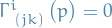 .
.
Hence, for a torsionless connection, this reduces to  .
.
Therefore, the Riemann tensor in normal coordinates at is simply
Due to anti-symmetry in the last two indices,
![\begin{equation*}
\tensor{R}{^{a}_{[bcd]}} = \frac{1}{3} \big( \tensor{R}{^{a}_{bcd}} + \tensor{R}{^{a}_{cdb}} + \tensor{R}{^{a}_{dbc}} \big)
\end{equation*}](../../assets/latex/general_relativity_1e08ec039f1f1d8e061d891ba6e93e25df445ddf.png)
Substituting in the above identity (since we are in normal coordinates),
![\begin{equation*}
\tensor{R}{^{a}_{[bcd]}} = \frac{1}{3} \big( \partial_c \tensor{\Gamma}{^{a}_{bd}} - \partial_d \tensor{\Gamma}{^{a}_{bc}} + \partial_d \tensor{\Gamma}{^{a}_{cb}} - \partial_b \tensor{\Gamma}{^{a}_{cd}} + \partial_b \tensor{\Gamma}{^{a}_{dc}} - \partial_c \tensor{\Gamma}{^{a}_{db}} \big) = 0
\end{equation*}](../../assets/latex/general_relativity_7a48494a5fbc36c070c4071381291de0115c3ee3.png)
since
 .
.
We have
So we need the last term to equal
 . To see this we write the expressions out
as we wanted. Substituting into the expression above,

as claimed.
![\begin{equation*}
\nabla_{[c} \tensor{R}{^{a}_{|b|de]}} = 0
\end{equation*}](../../assets/latex/general_relativity_bf72beb7eab9dbc9f36a1d673062b7602cb92dc4.png)
![\begin{equation*}
\begin{split}
\nabla_{[c} \tensor{R}{^{a}_{|b| de]}} &= \frac{1}{6} \Big( \nabla_c \tensor{R}{^{a}_{bde}} - \nabla_c \tensor{R}{^{a}_{bed}} + \nabla_e \tensor{R}{^{a}_{b cd}} - \nabla_e \tensor{R}{^{a}_{bdc}} + \nabla_d \tensor{R}{^{a}_{b ec}} - \nabla_d \tensor{R}{^{a}_{b ce}} \Big) \\
&= \frac{1}{3} \Big( \nabla_c \tensor{R}{^{a}_{bde}} + \nabla_e \tensor{R}{^{a}_{b cd}} + \nabla_d \tensor{R}{^{a}_{b ec}} \Big)
\end{split}
\end{equation*}](../../assets/latex/general_relativity_76ee9e18379884ce8bb500474dec92388d32ddc5.png)
which follows directly from
Then observe that

since in normal coordinates we have

because 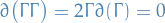 since
since  . Finally, substituting this into the above expression:
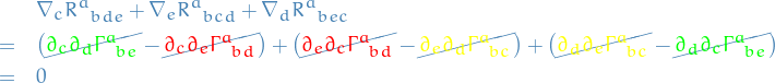
since partials commute.
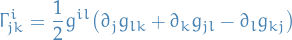
Levi-Civita connection
Let  be a psuedo-Riemannian manifold. There exist a unique connection with vanishing torsion and satisfying
  .
.
This choice of connection is often called the Levi-Civita connection.
Curvature of Levi-Civita connection
Let be the Levi-Civita connection. We define the (0, 4)-tensor


We work in normal coordinates at , so

and so
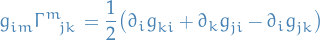
(at ) differentiate wrt.  and evaluate at :
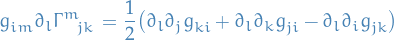
at .
AND MORE.

for Levi-Civita connection.

using Proposition proposition:4.61-lectures.
The Ricci scalar of  is
is
The Einstein tensor
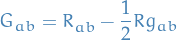


 , noting that
  by
by 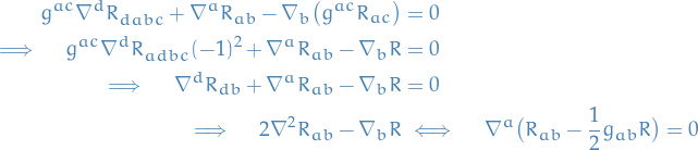
Riemann tensor of vanishes if and only if for every , there exists a chart containing such that
Recall if torsion vanishes, then Riemann tensor vanishes if and only if there exists charts where  . Then

in such charts.
This implies that  is constant in chart, if we choose basis at to be orthonormal, which implies
Theorem thm:Riemann-tensor-vanish-iff-Euclidean-or-Minkowski-metric shows us that the Riemann tensor sort of measure the deviation from Euclidean or Minkowski metric, locally.
Weyl tensor
- Ricci tensor and Ricci scalar contain information about "traces" of the Riemann tensor
- Sometimes useful to consider separately those parts of the Riemann tensor
 which the Ricci tensor
  does not tell us about
The Weyl tensor is defined (in  dimensions)
![\begin{equation*}
\tensor{C}{^{}_{abcd}} = \tensor{R}{^{}_{abcd}} - \frac{2}{(n - 2)} \big( \tensor{g}{^{}_{a [c}} \tensor{R}{^{}_{d] a}} - \tensor{g}{^{}_{b [c}} \tensor{R}{^{}_{d] a}} \big) + \frac{2}{(n - 1)(n - 2)} R \tensor{g}{^{}_{a[c}} \tensor{g}{^{}_{d]c}}
\end{equation*}](../../assets/latex/general_relativity_dd2fc54c0d56de307e015518185587e2553e3ef3.png)
The Weyl tensor is basically the Riemann tensor with all of its contractions removed. The above formula is designed so that all possible contractions of  vanish, while it retains the symmetries of the Riemann tensor:
![\begin{equation*}
\begin{split}
C_{abcd} &= C_{[ab][cd]} \\
C_{abcd} &= C_{cd ab} \\
C_{a [bcd]} &= 0
\end{split}
\end{equation*}](../../assets/latex/general_relativity_51bec12508fef6c7284ea63804215a4ab9dc1fb5.png)
One of the most important properties of the Weyl tensor is that it's invariant under
Special relativity
Spacetime is just a Lorentizan manifold  (Minkowski spacetime),
where
and  are the inertial coordinates, i.e.
  .
.
Free motion: are timelike geodesics, ligthrays null geodesics
Physics: described by tensor fields on which obey evolution equations.
Examples
Scalar field
Let  be a scalar field, then
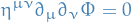
which is just the wave-equation:
![\begin{equation*}
\bigg( - \pdv[2]{}{(x^0)} + \pdv[2]{}{(x^1)} + \dots \bigg) \Phi = 0
\end{equation*}](../../assets/latex/general_relativity_0733cbc9fb09fb947c3e6f329bc56b6e14333f31.png)
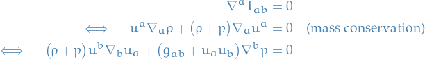
Energy-momentum tensor
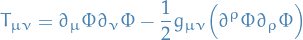
satisfies

which is conservation of energy / momentum.
Maxwell's theory of E. M.
Electromagnetic field strength
 which obeys the Maxwell's equations:
![\begin{equation*}
\tensor{\eta}{^{\mu \nu}_{}} \partial_{\mu} \tensor{F}{^{}_{\nu \rho}} = 0 \quad \text{and} \quad \partial_{[\mu} F_{\nu\ rho]} = 0
\end{equation*}](../../assets/latex/general_relativity_296481eddd2612a9d0b5c81001b1ce69d069d080.png)
The corresponding energy-momentum tensor

Any matter distribution is described by energy-momentum tensor
Fluids
- Described by vector field
 , and typically normalized such that
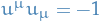
Perfect fluids:

where
- is the energy density
- is the pressure
- Then
 is the relativitic eqns. of fluid dynamics
General relativity
Main idea: there exist local freely flowing frames with no gravity.
This is achieved by the following postulates.
Postulates:
- Space-time is a 4D Lorentzian manifold
- Free particles follow timelike / null-geodesics wrt. Levi-Civita of
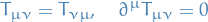
Energy-momentum distribution of matter fields described by
 symmetric tensor field
  which is conserved

The curvature of
is related to energy-momentum tensor of matter by the Einstein's equations:
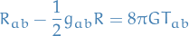
where
is the Newton gravitational constant.
- Note that might also depend on
 , so we cannot simply fix and solve
- Note that
Laws of physics governed by:
- General covariance: laws indep. of basis / coord system
- Equivalence principle: in any local inertial frame (normal coordinate system) laws reduce to the laws in Minkowski spacetime (Minkowski space)
Do not fix laws uniquely! But suggests simple rule (called minimal coupling):
given any equation in
(Minkowski space), we replace
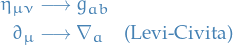
to get laws on curved spacetime
- Rules ensure general covariance as they output tensor equations.
Local intertial frames are normal coords at
, i.e.

Examples
Wave equation
Applying these rules to wave-equation of S.R. we get

 since
since  .
.
In local inertial frame, observe that we have

where the RHS is the wave-equation in .
Postulate 3: we have
and by wave-equation
Maxwell's equations
Applying these rules to Maxwell's equations in spacetime, we get
![\begin{equation*}
g^{ab} \nabla_a F_{bc} = 0 \quad \text{and} \quad \nabla_{[a} F_{bc]} = 0 \quad \text{and} \quad F_{ab} = - F_{ba}
\end{equation*}](../../assets/latex/general_relativity_fca23535160470786383a90a0d3f4178e4497eaf.png)
Postulate 3: we have
combined with Maxwell's equations we get
Fluids
- Described by vector field , and typically normalized such that
Perfect fluids:

where
- is the energy density
- is the pressure
Then
Motion of fluid given by
Observe that if the pressure vanish, i.e.  , then we're left with
which is the equation describing geodesic, fluid moves as "free particles".
Einstein's equations
- Motivation:
- Newtonian
- Graviational field described by scalar potential

Equation of motion

where
 in cartesian coordinates
Relative acceleration of nearby particles ("tildal force") governed by deviation equation
where
 is the separation vector of the particles
- Graviational field described by scalar potential
- GR:
Relative acceleration of two nearby particles following timelike geodesics is given by the geodesic deviation equation

where
 is the tangent to the geodesics and
  is now the deviation vector.
Comparison suggests

- Newtonian
Spacetimes
(anti-)de Sitter
de Sitter spacetime in  dimensions with radius of curvature
  is locally isometric to the quadratic

Anti de Sitter spacetime in dimensions with radius of curvature is locally isometric to the quadrics

More precisely, the de Sitter spacetimes are the simply-connected universal covers of these quadrics.
Taking the limit  is equivalent to the zero curvature limit in which we recover Minkowski spacetime.
The real affince space  with a metric which, when expressed relative to affine coordinates, is given by

where we have introduced the speed of light  .
.
We may take limits:
- non-relativistic limit (on the co-metric):
 gives us galilean spacetime
 - ultra-relativistic limit (on the co-metric):
 gives us carrollian spacetime
These spacetimes are no longer lorentzian: the (co-)metric becomes degenerate in the limit, leading to a galilean and a carrollian structure, respectively.