Fields
Table of Contents
Equations / Laws
Coulomb's Law
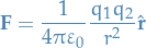 1
1
where permittivity constant of free space 
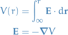
Electric Field

where  is the test charge,
  is the electric field at that point.
Magnetic Field

Lorentz Force
This is just writing the magnetic and electric in a single equation.

Electric Flux

Gauss's Law
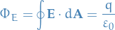
for Gaussian surfaces, i.e. general closed surface with all surface elements pointing outwards.
Potential Difference as work
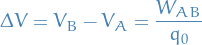
I.e. potential-difference is simply work used on a test-charge.
Potential Energy

Potential
Ampere's Law

Biot-Savarts
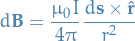
where  is the vector whose magnitude is the length of the
differential element of the wire in the direction of conventional
current.
is the vector whose magnitude is the length of the
differential element of the wire in the direction of conventional
current.
Thus,  is tangential to the surface of the wire,
perpendicular to the current-flow (following the right-hand rule).
is tangential to the surface of the wire,
perpendicular to the current-flow (following the right-hand rule).
Dipole moment
 2
2
where  is the distance between charges and
  is the dipole axis.
Continuous Charge Distribution
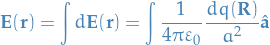
where 
Torque

Faraday's Law
Induced emf in a conducting loop is given by the rate of change of magnetic flux through the loop, i.e.

Lenz's Law
The induced current has a direction s.t. the magnetic field due to this current opposes the change in the magnetic field that caused it.
Capacitor
Charge stored

Impedence
Definitions
Electric dipole
Two charges of different charge separated by a fixed distance.
Examples
AC
Electromagnetic force  is given by:

The resulting current is:

where  is the phase-difference between and
  .
.
How-to
- Setup the differential equation for charge wrt. time, using Kirchoff's Law and the fact that the potential difference across all components need to sum to the potential difference across the entire circuit.
- Solve said differential equations.
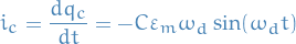
Capacitive load circuit

Thus, "current" across the capacitor