Quantum Mechanics
Table of Contents
2. A First Approach to Classical Mechanics
2.5 Poisson Brackets and Hamiltonian Mechanics
Let  and
and  be two smooth functions on
  , where an element of is thought of as a pair
  , with
 representing position of a particle
 representing the momentum of a particle
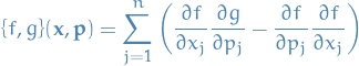
Then the Poisson bracket of and , denoted  is the function on given by
For all smooth functions , and  on we have the following:
 for all


Jacobi identity:

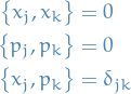
The position and momentum functions satisfy the following Poisson bracket relations:
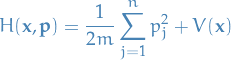
If a particle in  has the usual sort of energy function (kinetic energy plus potential energy), we have
Wit the Hamiltonian, and as usual, having  , we can write Netwon's laws as:
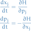
These equations we refer to has Hamilton's equations.
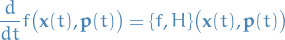
If  is a solution of the Hamilton's equation, then for any function on , we have
Call a smooth function on a conserved quantity if  is independent of
  for each solution of Hamilton's equations.
Then is a conserved quantity if and only if

In particular, the Hamiltonian  is a conserved quantity.
Solving Hamilton's equatons on gives rise to a flow on , that is, a family  of diffeomorphisms of , where
  is equal to the solution at time of Hamilton's equations with initial conditions .
Since it is possible (depending on the choice of potential function  ) that a particle can escape to infinity in finite time, the maps are not necessarily defined on all of , but only on some subset therof.
If is defined on all of we say it's complete.
The flow associated with Hamilton's equations, for an arbitrary Hamitonian function , preserves the (2n)-dimensional volume measure

What this means, more precisely, is that if a measurable set  is contained in the domain of for some
  , then the volume of
  is equal to the volume of .