Optimal Transport
Table of Contents
Discrete case
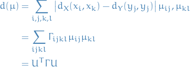
So the optimal transport problem becomes

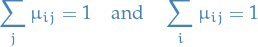
subject to linear constraints
villani09_optim_trans
7. Displacement interpolation
Notation
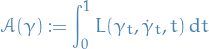
 denotes the action functional
 is a certain class of continuous curves
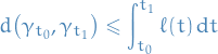
Cost function between an initial point
 and final point
  :
:

- Riemannian manifold

- Langrangian
 is defined on
 ![$TM \times [0, 1]$](../../assets/latex/optimal_transport_0ebea118dbffa116547361eb4b86307e074f66cb.png)
Deterministic interpolation via action-minimizing curves
Action is classically given by the time-integral of a *Lagrangian$ along the path:
A continuous curve
![$\gamma: [0, 1] \to \mathcal{X}$](../../assets/latex/optimal_transport_130876f47e1f6264d6518b489196576d03a24ea9.png) is absolutely continuous if there exists a function
is absolutely continuous if there exists a function ![$\ell \in L^1 \big( [0, 1]; \dd{t} \big)$](../../assets/latex/optimal_transport_5eb03540cb3f1d1d7670cccc143d5a4ef4821fd3.png) s.t. for all intermediate times
s.t. for all intermediate times  in
in ![$[0, 1]$](../../assets/latex/optimal_transport_68c8fa38d960e53d4308cbf1e65d04c66a554817.png) ,
,
- If
 is absolutely continuous, then
  is differentiable a.e. and its derivative is integrable.
- If
Examples
Let

 be a curve from
  to
to 
 for some strictly convex
Then, by Jensen's inequality,
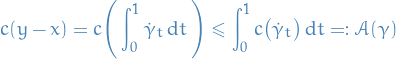
which is an equality only when  , and thus the action minimizers are lines , i.e. straight lines:

Also, then we have

since the cost function is defined by the minimizers of  .
.
Interpolation of random variables
- is a cost function associated with the Lagrangian action
 be two given laws
- Optimal coupling
 of
of 
- Random action-minimizing path
 joining
  to
to 
- => random variable
 is an interpolation of and ; or equivalently
  is an interpolation of
  and
and 
- This is referred to as displacement interpolation
This should be constrasted with linear interpolation

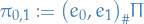
- A dynamical transference plan
 is a probability measure on the space
 ![$C \big( [0, 1]; \mathcal{X} \big)$](../../assets/latex/optimal_transport_31649c06ae9c3ec23a274ff3d882cffc6a90fb4a.png) (i.e. space of curves).
(i.e. space of curves). - A dynamical coupling of two probability measures
 is a random curve s.t.
  and
and  .
. A dynamical optimal transference plan is a prob. measure on
on  s.t.
s.t.
- Equivalently, is the law of a random action-minimizing curve whose endpoints constitute an optimal coupling of
 .
. - Such a random curve is called a dynamic optimal coupling of .
- By abuse of language, is sometimes referred to as the same.
- By abuse of language,
- Equivalently,