Linear Programming

Overview
Notation
From the basics
Introduction
Fourier-Motzkin Elimination
Equational / canonical form
TODO LP and reduction
- Solving LP (given feasible)
Basic feasible solution
TODO Initial BFS
TODO Simplex method
- Selecting an entering variable (to the basis)
- Simplex Tableau
Duality
Sources

Overview

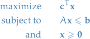
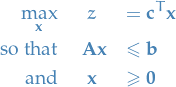
Linear programming is a technique for the optimization of a linear objective function, subject to linear equality and linear inequality constraints.

It's feasible region is a convex polytope.

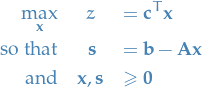
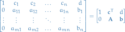
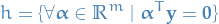
Linear programs are problems that can be expressed in canonical fomr as:

$\begin{equation*} \begin{split} \text{maximize} \qquad & \mathbf{c}^T \mathbf{x} \\ \text{subject to} \qquad & A \mathbf{x} \le \mathbf{b} \\ \text{and} \qquad & \mathbf{x} \ge \mathbf{0} \end{split} \end{equation*}$

Notation

$\mathbf{x}$ denotes the vector of variables
$\mathbf{c}$ and $\mathbf{b}$ are vectors of known coefficients
$m$ is # of constraints
$n$ is # of variables
$i \in [m]$ and $j \in [n]$ where $[n] = \{ 1, 2, \dots, n \}$
$K$ denotes the set of feasible / possible solutions

From the basics

Consider the following LP problem:

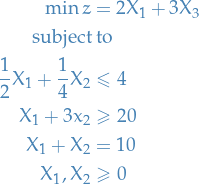
$\begin{equation*} \begin{split} \min z &= 2 X_1 + 3 X_3 \\ \text{subject} & \text{ to} \\ \frac{1}{2} X_1 + \frac{1}{4} X_2 & \le 4 \\ X_1 + 3 x_2 & \ge 20 \\ X_1 + X_2 & = 10 \\ X_1, X_2 & \ge 0 \end{split} \end{equation*}$

Then observe the following:

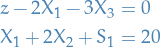
We an rewrite the objective:

$\begin{equation*} \min_{X_i} z = 2 X_1 + 3 X_2 \iff \min_{X_i} z - 2X_1 - 3X_2 = 0 \end{equation*}$

I.e., minimizing $z$ corresponds to finding $X_1$ and $X_2$ such that the smallest value $z$ can take on and still satisfy the equality is as small as possible!
We can rewrite an equality of the form

$\begin{equation*} X_1 + 2 X_2 \ge 20 \iff X_1 + 2 X_2 + S_1 = 20 \quad S_1 \ge 0 \end{equation*}$

EXPLAIN THIS PROPERLY

If we do this for all inequalities, we observe that we're left with a simple linear system:

$\begin{equation*} \begin{split} z - 2 X_1 - 3 X_3 &= 0 \\ X_1 + 2 X_2 + S_1 &= 20 \end{split} \end{equation*}$

Which we can simply solve using the standard Linear algebra! There are a couple of problems here though;

Not encoding the minimization of the objective
Not encoding the fact that the variables are non-negative (positive or zero)
If $m \le n$ , i.e. have more variables than constraints, then we have multiple possible solutions

Therefore we have to keep track of these two points ourselves;

The Simplex Method is a method which helps us with exactly that by doing the following:

Gives us certain conditions which have to be true if the solution we're currently considering is hte best solution we can in fact obtain
How to obtain other solutions given the solution we're currently considering (where we can just check which one is the best one by comparing the values $z$ takes on for the different solutions)

To address the first point: "how do we know that the solution under consideration is best ?" we make the following observation

then will have the best possible value of if , right?
- Since the coefficients of $X_1$ and $X_2$ are both negative, then any increase in the values of $X_1$ and $X_2$ will lead to decrease in the objective function $z$ !

The Simplex method makes use of this fact by observing that if we can transform the system of linear equations such that the coefficients of $X_i$ are all

Introduction

We are given an input of the following $m$ constraints (inequalities):

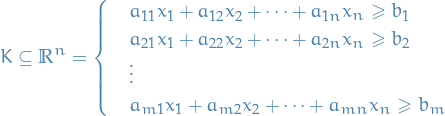
$\begin{equation*} K \subseteq \mathbb{R}^n = \begin{cases} & a_{11} x_1 + a_{12} x_2 + \dots + a_{1n}x_n \ge b_1 \\ & a_{21} x_1 + a_{22} x_2 + \dots + a_{2n}x_n \ge b_2 \\ & \vdots \\ & a_{m1} x_1 + a_{m2} x_2 + \dots + a_{mn}x_n \ge b_m \\ \end{cases} \end{equation*}$

where $a_{ij}, b_i \in \mathbb{Q}$ for $i \in [m]$ and $j \in [n]$ . And then we have some (linear) objective function we want to optimize wrt. $\mathbf{x} \in K$ , i.e. $\mathbf{x}$ such that the above constraints are satisfied.

Can always change the "direction" of the inequalities by simply multiplying one side by -1.

Also allow equality since

$\begin{equation*} \mathbf{a} \cdot \mathbf{x} = \mathbf{b} \iff \mathbf{a} \cdot \mathbf{x} \ge \mathbf{b} \wedge \mathbf{a} \cdot \mathbf{x} \le \mathbf{b} \end{equation*}$

but NOT strict inequalities!

Fourier-Motzkin Elimination

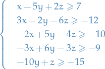
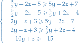
Let's do an example: assume that we're working with a 3-variable 5-constraint LP, namely,

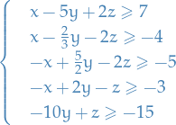
$\begin{equation*} \begin{cases} & x - 5y + 2z \ge 7 \\ & 3x - 2y - 6z \ge - 12 \\ & -2x + 5y - 4z \ge - 10 \\ & -3x + 6y - 3z \ge - 9 \\ & -10y + z \ge - 15 \end{cases} \end{equation*}$

Fourier-Motzkin elmination is then to recursively eliminate one of the variables. Let's do $x$ first:

"Normalize" the constraints wrt. $x$ , i.e. multiply constraints by constants such that coeff. of $x$ is in $\{ -1, 0, 1 \}$

$\begin{equation*} \begin{cases} & x - 5y + 2z \ge 7 \\ & x - \frac{2}{3} y - 2 z \ge -4 \\ & -x + \frac{5}{2} y - 2z \ge - 5 \\ & - x + 2y - z \ge -3 \\ & -10y + z \ge - 15 \end{cases} \end{equation*}$
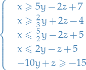
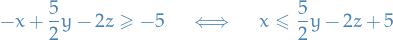
Write inequalities as:

$\begin{equation*} x \ge c_i y + d_i z + e_i \quad \text{or} \quad x \ge c_i y + d_i z + e_i \end{equation*}$

for some $c_i, d_i, e_i \in \mathbb{Q}$ depending on whether $x$ has coefficient $1$ or $-1$ (if coeff is 0, we just leave it). Then we get,

$\begin{equation*} \begin{cases} & x \ge 5y - 2z + 7 \\ & x \ge \frac{2}{3} y + 2z - 4 \\ & x \le \frac{5}{2} y - 2z + 5 \\ & x \le 2y - z + 5 \\ & -10y + z \ge - 15 \end{cases} \end{equation*}$

where we for example have done:

$\begin{equation*} - x + \frac{5}{2} y - 2z \ge - 5 \quad \iff \quad x \le \frac{5}{2}y - 2z + 5 \end{equation*}$
For each pair of "different" inequalities, we "combine" them to form:

$\begin{equation*} \begin{cases} & \frac{5}{2}y - 2z + 5 \ge 5y - 2z + 7 \\ & \frac{5}{2}y - 2z + 5 \ge \frac{2}{3}y + 2z - 4 \\ & 2y - z + 3 \ge 5y - 2z + 7 \\ & 2y - z + 3 \ge \frac{2}{3}y + 2z - 4 \\ & -10y + z \ge - 15 \end{cases} \end{equation*}$

Thus we have eliminated $x$ !
Repeat step 3 until we only have a single variable left, leaving us with a set of constraints for this last variable. If the constraints remaining cannot be satisfied by the remaining variable, then clearly this is an infeasible problem, i.e. $K = \emptyset$ .

Fourier-Motzkin Elimination actually solves the LP-problem; however, it does so incredibly inefficiently. As we'll see later, these problems can be solved in polynomial time.

FM elimination start out with $k$ inequalities, and in the worst case we end up with $k^2 / 4 = \Theta(k^2)$ new inequalities (due to pairing up all the "different" inequalities).

Equational / canonical form

We can constrain every variable $x_i$ to be $x_i \ge 0$ by introducing two variables $x_i^-, x_i^+$ for each variable $x_i$ . Then replace each occurence of $x_i$ by $(x_i^+ - x_i^-)$ and add the constraints $x_i^+ \ge 0, x_i^- \ge 0$ .

In doing so we end up with a positive orthant in $\mathbb{R}^n$ and constraints $A \mathbf{x} = \mathbf{b}$ is a $(n - m)$ dimensional subspace of $\mathbb{R}^n$ .

TODO LP and reduction

Solving LP (given feasible)

First we want to find Suppose $K \ne \emptyset$ . Then we only need to find $d_1, d_2, \dots, d_n \in \mathbb{Q}$ such that

$\begin{equation*} K \cap \{ x_i = d_i, \forall i \in [n] \} \ne \emptyset \end{equation*}$

i.e. some feasible solution $\mathbf{x} = \mathbf{d}$ .

We also assume that the feasible set is /bounded/¹, where $x_i \in [B_i^-, B_i^+]$ . We then use binary search to

Basic feasible solution

In geometric terms, the feasible region defined by all values of $\mathbf{x}$ such that

$\begin{equation*} \mathbf{A} \mathbf{x} = \mathbf{x}, \quad x_i \ge 0 \end{equation*}$

is a (possibly unbounded) convex polytope. There is a simple characterization of the extreme points or vertices of this polytope, namely an element $\mathbf{x} = (x_1, \dots, x_n)$ of the feasible region is an extreme point if and only if the subset of column vectors $\mathbf{A}_i$ corresponding to the non-zero entries of $\mathbf{x}$ ( $x_i \ne 0$ ) are linearly independent.

In this context, such a point is know as a basic feasible solution (BFS).

The BFS will always be of the same dimension as the number of constraints. That is,

$\begin{equation*} \dim B = m \end{equation*}$

since the number of constraints determines the number of independent variables in our system. Why? Well, if we have 3 variables and 2 constraints, then that means that one of the variables, say $x_1$ , can be expressed as a function of one of the other variables, say $x_2$ , and so on.

What does this mean? We can obtain some initial BFS by setting enough variables to zero such that we're left with only $m$ variables (where we should have only one variable being non-zero in each constraint). In this way we obtain some linearly indep. system from which we can start pivoting.

We call the variables currently in the basis basic variables, and those not in the basis non-basic variables.

TODO Initial BFS

If all the constraints in the original LP formulation are of the $\le$ type, we can readily obtain an initial BFS for Simplex, consisting of all the slack variables in the corresponding standard form formulation
Need to find an initial BFS, since we might not start with a matrix which has perpendicular columns (i.e. the columns are not orthonormal)

Consider the following general linear problem:

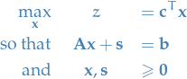
which in "standard form" becomes

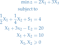
$\begin{equation*} \begin{split} \min z &= 2 X_1 + 3 X_3 \\ \text{subject} & \text{ to} \\ \frac{1}{2} X_1 + \frac{1}{4} X_2 + S_1 & = 4 \\ X_1 + 3 x_2 - E_2 & = 20 \\ X_1 + X_2 & = 10 \\ X_1, X_2 & \ge 0 \end{split} \end{equation*}$

where we've turned the inequalities into equalities by introducing slack-variables $S_1$ and $E_2$ .

$E_2$ cannot be a basic variable (included in the basis) for $C_2$ , even though it appears only in this constraint, since it would imply a negative value for it (i.e. $E_2 = -20$ ), and the resulting basic solution would not be feasible
$C_3$ does not even include an auxillary variable

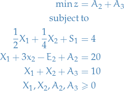
To fix these two problematic constraints $C_2$ and $C_3$ we "synthesize" an initial BFS by introducing additional artifical variables $A_2$ and $A_3$ for $C_2$ and $C_3$ , with $A_2, A_3 \ge 0$ .

Initial BFS is $B_0 = \{ S_1, A_2, A_3 \}$ with $S_1 = 4, \ A_2 = 20, \ A_3 = 10$
This alters the structure, and therefore the content, of the original LP
Easy to check that this BFS $B_0$ (together with the implied zero values of the nonbasic variables) is not feasible for the original LP!
BUT, if we obtain another BFS for the modified problem in which the artifical variables are non-basic , then this BFS would also be feasible for the original LP (since the artifical variables, being nonbasic, would be zero in the "canonical form")

To get artifical variables $A_2, A_3$ to zero, we try to achieve the following objective:

$\begin{equation*} \begin{split} \min z &= A_2 + A_3 \\ \text{subject} & \text{ to} \\ \frac{1}{2} X_1 + \frac{1}{4} X_2 + S_1 & = 4 \\ X_1 + 3 x_2 - E_2 + A_2 & = 20 \\ X_1 + X_2 + A_3 & = 10 \\ X_1, X_2, A_2, A_3 & \ge 0 \end{split} \end{equation*}$

This is known as Phase 1 of the Simplex method. Observe

If original LP has a feasible solution, then nonnegativity of and implies optimal value for altered LP will be zero!
- Hence, at the end of this altered LP we will have a feasible solution for the original formulation!
If, due to the strictly positive optimal objective value for altered LP, artifical variables $A_2, A_3$ are absolutely necessary to obtain a feasible solution for this set of constraints => original LP is infeasible

Therefore, all we do is solve the altered system, and if we get a solution for this without the introduced artifical variables $A_2, A_3$ in the BFS, we have an initial BFS for the original LP!

TODO Simplex method

Have an LP in (primal) form:

$\begin{eqnarray*} \max_{\mathbf{x}} & z &= \mathbf{c}^T \mathbf{x} \\ \text{so that} & \ \mathbf{A} \mathbf{x} & \le \mathbf{b} \\ \text{and} & \mathbf{x} & \ge \mathbf{0} \end{eqnarray*}$

Note the inequality of constraints.

Add slack variables $s_i$ to each inequality, to get:

$\begin{eqnarray*} \max_{\mathbf{x}} & z &= \mathbf{c}^T \mathbf{x} \\ \text{so that} & \ \mathbf{A} \mathbf{x} + \mathbf{s} & = \mathbf{b} \\ \text{and} & \mathbf{x}, \mathbf{s} & \ge \mathbf{0} \end{eqnarray*}$

Why bother?
- We're now left with the familiar (primal) form of a LP
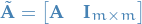
  - To make it completely obvious, one can let $s_i = x_{n + i}$ and add the identity matrix to the lower-left of the matrix $\mathbf{A}$
    
    $\begin{equation*} \tilde{\mathbf{A}} = \begin{bmatrix} \mathbf{A} & \mathbf{I}_{m \times m} \end{bmatrix} \end{equation*}$
    
    Then we can write the problem with slack-variables as a system of linear equations:
    
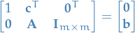
    $\begin{equation*} \begin{bmatrix} 1 & \mathbf{c}^T & \mathbf{0}^T \\ \mathbf{0} & \mathbf{A} & \mathbf{I}_{m \times m} \end{bmatrix} = \begin{bmatrix} \mathbf{0} \\ \mathbf{b} \end{bmatrix} \end{equation*}$
- Every equality constraint now has at least one variable on the LHS with coeff. 1, which is indep. of the other inequalities
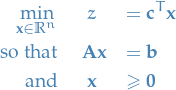
- Picking one such variable for each equality, we obtain a set $B$ of $m$ variables called a basis (variables in the basis are called basic variables); an obvious choice is
  
  $\begin{equation*} B = \{ s_1, \dots, s_m \} \end{equation*}$
Rearrange constraints to get

$\begin{eqnarray*} \max_{\mathbf{x}} & z &= \mathbf{c}^T \mathbf{x} \\ \text{so that} & \ \mathbf{s} & = \mathbf{b} - \mathbf{A} \mathbf{x} \\ \text{and} & \mathbf{x}, \mathbf{s} & \ge \mathbf{0} \end{eqnarray*}$

Just for the sake of demonstration, suppose all constraints are positive, i.e. $\mathbf{b} \ge 0$ . Then clearly the best solution is just letting $\mathbf{x} = 0$ . This then corresponds to a vertex.
Nowe we have some initial suggestion for a solution, i.e. a basic feasible solution (BFS) with basis $B$ . To find other possible solutions; pivot! Let the current basis be

$\begin{equation*} B = \{ x_{i_1}, x_{i_2}, \dots, x_{i_m} \} \end{equation*}$

with $x_{i_r}$ being a variable on the LHS of the r-th constraint $C_r$ (in the above rearrangement). We then suggest a new basis $B'$

$\begin{equation*} B' = \big( B \setminus \{ x_{i_r} \} \big) \cup \{ x_j \} \end{equation*}$

i.e. removing $x_{i_r}$ and choosing some other $x_j$ on the LHS of constraint $C_r$ , which is performed as follows:
1. Assuming $C_r$ involves $x_j$ , rewrite $C_r$ using $x_j = \alpha$
2. Substitute $x_j = \alpha$ in all other constraints $C_l$ , obtaining constraints $C_l'$
3. New constraints $C_l'$ have a new basis
  
  $\begin{equation*} B' = \big( B \setminus \{ x_{i_r} \} \cup \{ x_j \} \big) \end{equation*}$
4. Substitute $x_j = \alpha$ in the objective $f(x)$ so that $f(x)$ again only depends on variables not in basis

Of course, we're not going to pivot no matter what! We pivot if and only if:

New constants $\mathbf{b} \ge 0$ , since this is a boundary condition
New basis must at least not decrease objective function

Consider a new candidate basis:

$\begin{equation*} B' := \big( B \setminus \left\{ x_{i_r} \right\} \big) \cup \left\{ x_j \right\} \end{equation*}$

for some $x_j \not\in B$ , i.e.

Replace $x_{i_r}$ by $x_j$ where $x_j$ is non-basic variable currently used in constraint $C_r$
Rewrite cosntraint $C_r$ such that we get an expression for $x_j$

Selecting an entering variable (to the basis)

Given that at every objective-improving iteration the Simplex algorithm considers adjacent bfs's, it follows that only one candidate non-basic variable enters the basis
Want variable with greatest improvement to the objective to enter basis
For a variable to enter, we need one to leave:

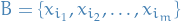
Simplex Tableau

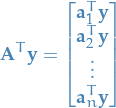
Take a LP-problem in primal form, we can write it as an augmented matrix with the following:

1st column corresponds to coefficent of $z$ (objective function)
2nd through n + 1 corresponds to coefficients of $x_i$ , i.e. $c_i$
Last (n + 2) column is the constant in the objective function and RHS of constraints

Then we can write

$\begin{equation*} \begin{bmatrix} 1 & c_1 & c_2 & \dots & c_n & d \\ 0 & a_{11} & a_{12} & \dots & a_{1n} & b_1 \\ \vdots & \vdots & \vdots & \ddots & \vdots & \vdots \\ 0 & a_{m1} & a_{m2} & \dots & a_{mn} & b_n \end{bmatrix} = \begin{bmatrix} 1 & \mathbf{c}^T & d \\ 0 & \mathbf{A} & \mathbf{b} \end{bmatrix} \end{equation*}$

where $d$ is simple the value $z$ takes on if all variables are zero, i.e.

$\begin{equation*} x_i = 0 \implies z = d \end{equation*}$

usually we set this to zero, $d = 0$ .

Now, this is just a linear system, for which there exists

if : independent variables
- when we've solved for the $m$ constraints, the rest of the variables are simply functions of the constraints
if $n \le m$ : $n$ independent variables (might not be able to satisfy the constraints)

Now we simply make use of Gaussian Elimination to solve this system;

unless the matrix has linearly indep. columns and is $n \times n$ , we do not have a unique solution!
therefore we simply look for solutions where we have some $m$ linearly independent columns, which we say form our basis $B$ (see BFS)

<2018-02-05 Mon> But what if the $c_i$ are not all non-negative?!

They can't be yah dofus! You have optimality exactly when they are all non-negative.

If they're not, you pivot!

Duality

Notation

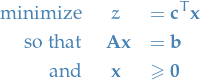
Linear problem (primary form)

$\begin{eqnarray*} \min_{\mathbf{x} \in \mathbb{R}^n} & z &= \mathbf{c}^T \mathbf{x} \\ \text{so that} & \ \mathbf{A} \mathbf{x} & = \mathbf{b} \\ \text{and} & \mathbf{x} & \ge \mathbf{0} \end{eqnarray*}$
$\mathbf{x}$ is the variables to minimize over
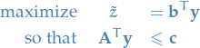
Linear problem (dual form)

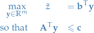
$\begin{eqnarray*} \max_{\mathbf{y} \in \mathbb{R}^m} & \tilde{z} & = \mathbf{b}^T \mathbf{y} \\ \text{so that} & \ \mathbf{A}^T \mathbf{y} & \le \mathbf{c} \end{eqnarray*}$

Primal form

$\begin{eqnarray*} \text{minimize} & z &= \mathbf{c}^T \mathbf{x} \\ \text{so that} & \ \mathbf{A} \mathbf{x} & = \mathbf{b} \\ \text{and} & \mathbf{x} & \ge \mathbf{0} \end{eqnarray*}$

Dual form

$\begin{eqnarray*} \text{maximize} & \tilde{z} & = \mathbf{b}^T \mathbf{y} \\ \text{so that} & \ \mathbf{A}^T \mathbf{y} & \le \mathbf{c} \end{eqnarray*}$

Weak Duality Theorem

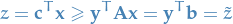
$\begin{equation*} z = \mathbf{c}^T \mathbf{x} \ge \mathbf{y}^T \mathbf{A} \mathbf{x} = \mathbf{y}^T \mathbf{b} = \tilde{z} \end{equation*}$

That is,

$\begin{equation*} z \ge \tilde{z} \end{equation*}$

Farkas Lemma

Let $\mathbf{A} \in \mathbb{R}^{m \times n}$ and $\mathbf{b} \in \mathbb{R}^m$ .

Then exactly one of the following statements is true:

There exists an $\mathbf{x} \in \mathbb{R}^n$ such that $\mathbf{A} \mathbf{x} = \mathbf{b}$ and $\mathbf{x} \ge 0$
There exists a $\mathbf{y} \in \mathbb{R}^m$ such that $\mathbf{A}^T \mathbf{y} \le 0$ and $\mathbf{b}^T \mathbf{y} > 0$

The way I understand Farkas lemma is as follows:

$\mathbf{b} \in \text{span}_{\mathbf{x} \ge \mathbf{0}} \big( \text{col}(\mathbf{A}) \big)$ , then clearly $\exists \mathbf{x} \ge \mathbf{0}$ such that $\mathbf{A} \mathbf{x} = \mathbf{b}$
$\mathbf{b} \in \text{span}_{\mathbf{x} \ge \mathbf{0}} \big( \text{col}(\mathbf{A}) \big)$ , then we can find some vector $\mathbf{y} \in \mathbb{R}^m$ such that the hyperplane defined by

$\begin{equation*} h = \{ \forall \boldsymbol{\alpha} \in \mathbb{R}^m \mid \boldsymbol{\alpha}^T \mathbf{y} = \mathbf{0} \} \end{equation*}$

i.e. $\mathbf{y}$ is the norm of $h$ , such that

$\begin{equation*} \mathbf{A}^T \mathbf{y} \le \mathbf{0} \quad \text{and} \quad \mathbf{b}^T \mathbf{y} > 0 \end{equation*}$

or, equivalently,

$\begin{equation*} \mathbf{A}^T \mathbf{y} \ge \mathbf{0} \quad \text{and} \quad \mathbf{b}^T \mathbf{y} < 0 \end{equation*}$

Where:

$\begin{equation*} \mathbf{A}^T \mathbf{y} = \begin{bmatrix} \mathbf{a}_1^T \mathbf{y} \\ \mathbf{a}_2^T \mathbf{y} \\ \vdots \\ \mathbf{a}_n^T \mathbf{y} \end{bmatrix} \end{equation*}$

From now on, we'll use the notation $\text{col}(\mathbf{A})$ . Now, what if we decided to normalize each of these $\mathbf{a}_i$ ? Well, then we're looking at the the projection of $\mathbf{y}$ onto the ${col}(\mathbf{A})$ . Why is this interesting? Because the inequality

$\begin{equation*} \mathbf{A}^T \mathbf{y} \le \mathbf{0} \end{equation*}$

is therefore saying the the projection of $\mathbf{y}$ onto $\text{col}(\mathbf{A})$ , is non-positive in all entries, i.e. the angle between $\mathbf{y}$ and all vectors in $\text{col}(\mathbf{A})$ / is $\theta \in [\frac{\pi}{2}, \pi)$ !!! (including the full In turn, this implies that the hyperplane $h$ , which is defined by all vectors perpedincular to $\mathbf{y}$ , i.e. angle of $\frac{\pi}{2}$ , lies "above" $\text{col}(\mathbf{A})$ , since $\theta - \frac{\pi}{2} \in [0, \frac{\pi}{2})$ . Finally, we're computing $\mathbf{b}^T \mathbf{y}$ , which is obtaining the angle between the $\mathbf{b}$ and $\mathbf{y}$ . Then saying that

$\begin{equation*} \mathbf{b}^T \mathbf{y} > 0 \end{equation*}$

is equiv. of saying that the angle between $\mathbf{b}$ and $\mathbf{y}$ is $\varphi \in (0, \frac{\pi}{2})$ . BUT, if $\mathbf{b}$ is an angle of $\varphi \in (0, \frac{\pi}{2})$ wrt. $\mathbf{y}$ , AND $\mathbf{y}$ is an angle $\theta \in [\frac{\pi}{2}, \pi)$ with $\text{col}(\mathbf{A})$ . Then, since the hyperplane $h$ is at $\frac{\pi}{2}$ wrt. $\mathbf{y}$ , then $\mathbf{b}$ lies somewhere between $\mathbf{y}$ and the hyperplane $h$ , which in turn lies above $\text{col}(\mathbf{A})$ , hence $h$ lies between $\text{col}(\mathbf{A})$ and $\mathbf{b}$ .

Strong Duality

The optimal (maximal) value for the dual form of a LP problem is also the optimal (minimal) value for the primal form of the LP problem.

Let the minimal solution to the primal problem be

$\begin{equation*} z^* = \mathbf{c}^T \mathbf{x}^* \end{equation*}$

Then define

$\begin{equation*} \hat{\mathbf{A}} = \begin{bmatrix} \mathbf{A} \\ - \mathbf{c}^T \end{bmatrix}, \quad \hat{\mathbf{b}}_{\varepsilon} = \begin{bmatrix} \mathbf{b} \\ - z^* + \varepsilon \end{bmatrix}, \quad \hat{\mathbf{y}} = \begin{bmatrix} \mathbf{y} \\ \alpha \end{bmatrix} \end{equation*}$

with $\varepsilon, \alpha \in \mathbb{R}$ . We then have two cases for $\varepsilon$ :

$\varepsilon = 0$ , in which case we 1. of Farkas lemma because $\hat{\mathbf{A}} \mathbf{x}^* = \hat{\mathbf{b}}_0$

$\begin{equation*} \begin{bmatrix} \mathbf{A} \\ - \mathbf{c}^T \end{bmatrix} \mathbf{x}^* = \begin{bmatrix} \mathbf{A} \mathbf{x}^* \\ - \mathbf{c}^T \mathbf{x}^* \end{bmatrix} = \begin{bmatrix} \mathbf{b} \\ - z^* \end{bmatrix} = \hat{\mathbf{b}}_0 \end{equation*}$
$\varepsilon > 0$ , in which case there exists no non-negative solution (because $z^*$ is already minimal) and we have Farkas lemma case 2. Thus, there exist $\mathbf{y}$ and $\alpha$ , such that

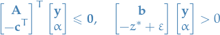
$\begin{equation*} \begin{bmatrix} \mathbf{A} \\ - \mathbf{c}^T \end{bmatrix}^T \begin{bmatrix} \mathbf{y} \\ \alpha \end{bmatrix} \le \mathbf{0}, \quad \begin{bmatrix} \mathbf{b} \\ - z^* + \varepsilon \end{bmatrix} \begin{bmatrix} \mathbf{y} \\ \alpha \end{bmatrix} > 0 \end{equation*}$

or, equivalently,

$\begin{equation*} \mathbf{A}^T \mathbf{y} \le \alpha \mathbf{c}, \quad \mathbf{b}^T \mathbf{y} > \alpha (z^* - \varepsilon) \end{equation*}$

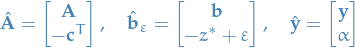
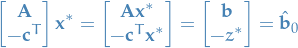
Now, we can find $\hat{\mathbf{y}}$ such that

$\begin{equation*} \hat{\mathbf{b}}_0 \hat{\mathbf{y}} = 0 \end{equation*}$

Then, letting $\varepsilon > 0$ , from the equation above, we would get

$\begin{equation*} \hat{\mathbf{b}}_0 \hat{\mathbf{y}} > 0 \end{equation*}$

Which we observe is only possible if $\alpha > 0$ , since $z^* > 0$ . $\hat{\mathbf{y}}$ is simply the normal vector of the hyperplane, thus we can scale it arbitarily; let's set $\alpha = 1$ :

$\begin{equation*} \mathbf{A}^T \mathbf{y} \le \mathbf{c}, \quad \mathbf{b}^T \mathbf{y} > z^* - \varepsilon \end{equation*}$

Observe that

$\begin{equation*} \tilde{z} := z^* - \varepsilon, \quad \varepsilon > 0 \end{equation*}$

is a feasible value for the objective of our dual problem. From the Weak Duality Theorem, we know that

$\begin{equation*} \tilde{z} \le z^* \end{equation*}$

But, we've just shown that we can get arbitrarily close to $z^*$ , hence at optimality (maximal) value of our dual form we also have $z^*$ !!!