Timeseries modelling
Table of Contents
Autoregressive (AR)
Idea
Output variable depends linearly on its own previous values and on a stochastic term (accounting for the variance in the data).
Model
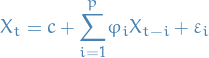
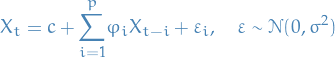
AR(p) refers to autoregressive model of order p, and is written
 1
1
where
 are parameters
 is a constant
 is white noise (Gaussian rv.), i.e.
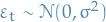
The unknowns are:
- constant
- the weights / dependence
 of the previous observations
 - the variance of the white noise

Estimating the parameters
- Ordinary Least Squares (OLS)
- Method of moments (through Yule-Walker equations)
There is a direct correspondance between the parameters
and the covariance of the process, and this can be "inverted" to
determine the parameters from the autocorrelation function itself.
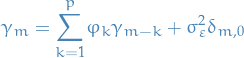
Yule-Walker equations
 2
2
where
 is the autocovariance function of
 is the std. dev. of the input noise process
 is the Kroenecker delta function, which is only non-zero when
Now, if we only consider  , we can ignore the last term, and can simply
write the above in matrix form:
, we can ignore the last term, and can simply
write the above in matrix form:
My thinking
Our plan is as follows:
- Consider each sequence of
 steps (the order of the
 AR) - Deduce distribution for conditioned on the parameters of the model
and the previous observations,
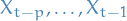 .
. - Obtain conditional log-likelihood function for this conditional distribution
- Get gradient of said conditional log-likelihood function
- Maximize said conditional log-likelihood wrt. parameters
- ???
- PROFIT!!!
Initial observation sequence
We start by collecting the first observations in a the sample  ,
writing it as
,
writing it as  , which as a mean vector
  where
where
 3
3
Why?
Well, we start out with the taking the expectation of  wrt. the random variables,
i.e. :
wrt. the random variables,
i.e. :
![\begin{equation*}
E[X_{p}] = E[c + \overset{p}{\underset{k=1}{\sum}} \varphi_i X_{p - i} + \varepsilon_{p}]
\end{equation*}](../../assets/latex/timeseries_modelling_246a72c6278eaf0be64984a15007f74899484c4e.png) 4
4
Then we start expanding:
![\begin{equation*}
\begin{split}
E[X_p] &= E[c] + E[\overset{p}{\underset{k=1}{\sum}} \varphi_i X_{p - i}] + E[\varepsilon_p] \\
&= c + \overset{p}{\underset{k=1}{\sum}} \varphi_i E[X_{p - i}] + 0, \quad E[\varepsilon_p] = 0 \\
&= c + \overset{p}{\underset{k=1}{\sum}} \varphi_i \mu \\
&= c + \mu \overset{p}{\underset{k=1}{\sum}}
\end{split}
\end{equation*}](../../assets/latex/timeseries_modelling_538f8ae1220f1082f853fd5c61fc3127bf8d641d.png) 5
5
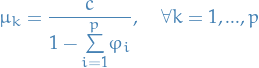
And since ![$E[X_p] = \mu$](../../assets/latex/timeseries_modelling_24e9a14e9ea05cd40ee1284326847555797b844b.png) , we rearrange to end up with:
, we rearrange to end up with:
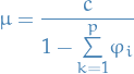 6
6
Voilá!
and the variance-covariance matrix is given by
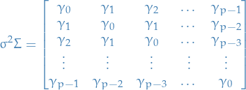 7
7
where  for two different steps
  and
and  .
This is due to the process being weak-sense stationary.
.
This is due to the process being weak-sense stationary.
The reason for the covariance matrix, is that by our assumption of weak-sense stationarity (is that a word? atleast it is now).
Conditional distribution
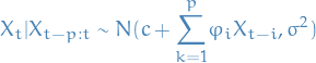
First we note the following:
 8
8
is equivalent of
 9
9
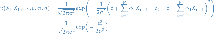
We then observe that if we condition on the previous observations,
it is independent on everything before that. That is;
 10
10
where  .
.
Therefore,
 11
11
For notational sake, we note that we can write it in the following form:
 12
12
We can write the total probability of seeing the data conditioned on the parameters as follows:
 13
13
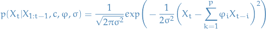
Which, when we substitute in the normal distributions obtained for ,
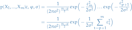 14
14
Conditional log-likelihood
Taking the logarithm of the previous expression, we obtain the conditional log-likelihood:
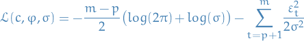 15
15
And just to remind you; what we want to do is find the parameters which maximizes the condition log-likelihood. If we frame it as a minimization problem, simply by taking then egative of the log-likelihood, we end up with the objective function:
 16
16
Now, we optimize!
Optimization
If we only consider the objective function wrt. to and , we end up with:
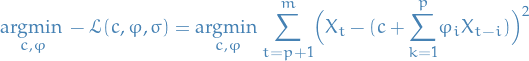 17
17
This is what I arrived at independently, but really thought this was a huge issue because
is defined as a function of the other variables and so we have a recursive relationship!
But then I realized, after confirming that the above is in fact what you want, that the
 in this equation are observed values, not random variables, duh!
Might be easier to think about it as
in this equation are observed values, not random variables, duh!
Might be easier to think about it as 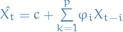 , and so we're looking at
  ,
since the last term is in fact our estimate for .
,
since the last term is in fact our estimate for .
Disclaimer: I think…
Thus, the conditional MLE of these parameters can be obtained from an OLS
regression of on a constant and of its own lagged values.
The conditional MLE estimator of turns out to be:
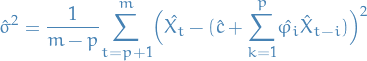 18
18
This can be solved with iterative methods like:
- Gauss-Newton algorithm
- Gradient Descent algorithm
Or by finding the exact solution using linear algebra, but the naive approach to this is quite expensive. There are definitively libraries which do this efficiently but nothing that I can implement myself, I think.
Moving average (MA)
Autoregressive Moving average (ARMA)
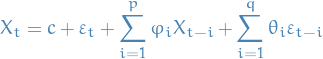
Arma(p, q) refers to the model with autoregressive terms and  moving-average terms. This model contains the AR(p) and MA(q) models,
Autoregressive Conditional Heteroskedasticity (ARCH)
Notation
- Heteroskedastic refers to sub-populations of a collection of rvs. having different variablility
Stuff
- Describes variance of current error term as a function of the actual sizes of the previous time periods' error terms
- If we assume the error variance is described by an ARMA model, then we have Generalized Autoregressive Conditional Heteroskedasticity (GARCH) model
Let denote a real-valued discrete-time stochastic process, and  and be the information set of all information up to time , i.e.
  .
.
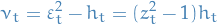
The process  is said to be a Autoregressive Conditional Heteroskedasticitic model or ARCH(q), whenever
![\begin{equation*}
\mathbb{E}[\varepsilon_t \mid \psi_{t - 1}] = 0 \quad \text{and} \quad \text{Var}(\varepsilon_t \mid \psi_{t - 1}) = h_t
\end{equation*}](../../assets/latex/timeseries_modelling_b666cc4f8454cf6c7ec5bd98b7781551aef6b67c.png)
with
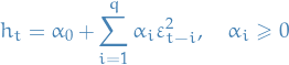
The conditional variance can generally be expressed as

where  is a nonnegative function of its arguments and
 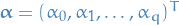 is a vector of unknown parameters.
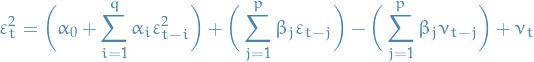
The above is sometimes represented as

with ![$\mathbb{E}[z_t] = 0$](../../assets/latex/timeseries_modelling_ebf30e825e3180c606b4438c6cacbe2c5c4d168a.png) and
and  , where the
  are uncorrelated.
We can estimate an ARCH(q) model using OLS.
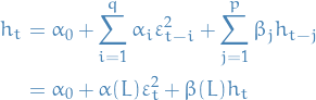
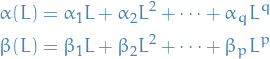
 and
and  are lag operators such that
Integrated GARCH (IGARCH)
Fractional Integrated GARCH (FIGARCH)
TODO Markov Switching Multifractal (MSM)
Useful tricks
Autocorrelation using Fourier Transform
Observe that the autocorrelation for a function  can be computed as follows:
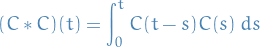
since this is just summing over the interactions between every value . If ![$C: [0, t] \to \mathbb{R}$](../../assets/latex/timeseries_modelling_358432e8ad6c30d4208a763a5ad4646d9679582e.png) , then the above defines the autocorrelation between the series, as wanted.
, then the above defines the autocorrelation between the series, as wanted.
Now, observe that the [BROKEN LINK: No match for fuzzy expression: def:fourier-transform] has the property:
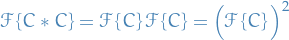
Hence,
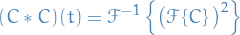
Which means that, given a dataset, we can use the efficient Fast Fourier Transform (FFT) to compute  , square it, and then take the inverse FFT, to obtain
  , i.e. the autocorrelation!
This is super-dope.
Appendix A: Vocabulary
- autocorrelation
- also known as serial correlation, and is the correlation of a signal with a delayed copy of itself as a function of delay. Informally, similarity between observations as a function of the time lag between them.
- wide-sense stationary
- also known as weak stationary, only require that the mean (1st moment) and autocovariance do not vary wrt. time. This is in contrast to stationary processes, where we require the joint probability to not vary wrt. time.