Strategic planning & classification
Table of Contents
Definitions
Pareto-optimal
If a solution to a game is Pareto-optimal, then a beneficial change for one agent is detrimental to another, i.e. we've reached a solution for which any change results in "inequality".
Pareto-optimality is different from Nash equilibrium (NE) because in a NE it's not profitable for any of the agents to change their strategy, but in Pareto-optimiality it can be beneficial for agents to change their strategy but it results in an "inbalance".
Pareto-optimalty is therefore often used in the context where you want everyone to do equally well, e.g. economics.
Idea
- Machine learning often relies on the assumption that unseen test instances of a classification problem follow the same distribution as observed data
- This can often break down when used to make decisions about the welfare of strategic individuals
- Knowing information about the classifier, such individuals may manipulate their attributes in order to obtain a better classification outcome
- Often referred to as gaming
- Result: performance of classifier may deteriorate sharply
- In financial policy-making this problem is widely known as Goodhart's law: "When a measure becomes a target, it ceases to be a good measure."
- Knowing information about the classifier, such individuals may manipulate their attributes in order to obtain a better classification outcome
- Strategic classification is an attempt to address this:
- Classification is considered as a sequential game between a player named
Juryand a player namedContestant Jurydesigns a classifierContestantmay change input based onJury's classifier- However,
Contestantincurs a cost for these changes, according to some cost function Jury's goal:- Achieve high classification accuracy wrt.
Contestant's original input and some underlying target classification function , assuming
 Contestantplays best response
- Achieve high classification accuracy wrt.
Contestant's goal:- Achieve a favorable classification (i.e. 1 rather than -1) while taking into account the cost of achieving it
- Classification is considered as a sequential game between a player named
Motivation
Examples
- Traffic predictions affect the traffic
Possible ideas
[ ]milli18_social_cost_strat_class suggests that there's a trade-off between the non-strategic equilibrium and the Stackelberg equilibrium- E.g. institution might only gain a very small increase in its utility while incurring a large social burden
- Could imagine constructing a utility function for the institution ("social planner") which makes explicit this trade-off
- Might be similar to rambachan2020economic
- Adding temporal dependence
- Current approaches does not have any notion of temporal dependence encoded
- Gaming vs. incentivized improvement could be combined by adding "short-term" cost function for gaming purpose and "long-term" cost for incentivized improvement
- Requires analysis similar-looking to bandits I would imagine?
- Could also try to design a classifier which "motivates" the agent to proritize the long-term rewards by incremental change
[ ]Generalize results from dong17_strat_class_from_reveal_prefer to work on convex problems with unbounded domain- Maybe possible to exploits some results from nesterov2017random, e.g.
- Proof of Theorem 2
- Maybe possible to exploits some results from nesterov2017random, e.g.
[ ]
General notes
- There are mainly two approaches to strategic adaptation:
- "Individuals try to game our classifier; can be construct a classifier which acts robustly even under gamification?"
- "Can we design classifiers that incentivize individuals to improve a desired quality?"
- Sequence of works
- Agents are represented by feature vectors which can be manipulated at a cost
- Problem: design optimal learning algo. in the presence of costly strategic manipulations of feature vector
- Gaming view hardt15_strat_class
- Manipulations do not change the underlying feature vector, only transforms the feature represented to the classifier → disadvantages the classifier
- Initial work: hardt15_strat_class
- Considers the problem as a two-player game, with one player being a binary classifier
- Extensions:
- Assume different groups of agents have different costs, and study disparate impact on their outcomes dong17_strat_class_from_reveal_prefer
- Learner does not know the distribution of agents features or costs but must learn them through revealed preference hu18_dispar_effec_strat_manip,milli18_social_cost_strat_class
- Improvement view
Notes for different papers
- hardt15_strat_class
- Follows approach (1)
- Formulates the problem of strategic classification as a sequential two-player game between a
Juryand aContestant:Jury's payoff:![\begin{equation*}
\mathbb{P}_{x \sim \mathcal{D}} \big[ h(x) = f \big( \Delta(x) \big) \big]
\end{equation*}](../../assets/latex/strategic_planning_7ddc7ee923687c6c3eea340ad953f17e46197a75.png)
Contestant's payoff:![\begin{equation*}
\mathbb{E}_{x \sim \mathcal{D}} \big[ f \big( \Delta(x) \big) - c \big( x, \Delta(x) \big) \big]
\end{equation*}](../../assets/latex/strategic_planning_ad82302ab9408c12f251ae7481861e20ab82c849.png)
- where
- is true classifier
 is
is Jury's classifier denotes the cost for the
 Contestant is the
 Contestant's "gaming-mechanism", in the sense that it tries to map to some positive example, i.e.
  , while balancing off the cost
- When using empirical examples from
 rather than full distribution , obtains result for separable cost functions, i.e.
  for functions
  s.t.
s.t. 
With prob
 , their algorithm (Algorithm 1)
  produces a classifier
  so that

with
 denoting the true optimally robust
- Generalize to arbitrary cost functions
- Is done by generalizing from separable cost functions to minimas for a set of separable cost functions
- Then show that all cost functions can be represented this way
- Drawback: bound scales with the size of the set of separable cost functions used, and thus quickly become not-so-useful
- They show that the problem is NP-hard for the case of general cost functions
- roth15_watch_learn
- miller19_strat_class_is_causal_model_disguis
- Any procedure for designing classifiers that incentivize improvement must inevitably solve a non-trivial causal inference problem
- Draw the following distinctions:
- Gaming: interventions that change the classification
 , but do not change the true label
- Incentiziving improvement: inducing agents to intervene on causal features that can change the label rather than non-causal features
- Gaming: interventions that change the classification
- haghtalab2020maximizing
- Thoughts:
- Not super-excited about this one. The most significant part of this paper focuses on obtaining “robust” linear threshold mechanisms under a lot of different assumptions, e.g. knowledge of the true classifier. A bit too specific IMO. Though I like the idea of finding approximately optimal mechanisms, where the “approximate” part comes from comparison to the gain in utility.
- Model is similar to hardt15_strat_class
- Instead of only considering a binary classifier, generalizes slightly allowing an arbitrary "scoring mechanism"
 , e.g.
![$g: \mathbb{R}^n \to [0, 1]$](../../assets/latex/strategic_planning_0d3d4162aa67e281f3ae25249f1eb68a6bcfce3b.png) representing the probability of the input being accepted
representing the probability of the input being accepted representing a binary-classification
 representing the payoff an individual receives (larger being better)
- Similarily to the "robust classifier" of hardt15_strat_class, they want to find some optimal scoring mechanism

- E.g. indicate overall health of an individual and
 the set of governmental policies on how to set insurance premium based on observalbe features of individuals
- Then
 corresponds to the policy that leads to the healthiest society on average
- Then
- E.g.
- Relating to hardt15_strat_class, is the true classifier (denoted ) and is the
Jury's classifier (denoted)
- Instead of only considering a binary classifier, generalizes slightly allowing an arbitrary "scoring mechanism"
- Consider only a subset of input-features to be visible, i.e. the mechanism only sees some projection
 of the true input
- This kind of emulates a causal structure, similar to what described in miller19_strat_class_is_causal_model_disguis
- Here they also add on a "smoothing" noise of the form
 with
with  , which is basically an instance of the exogenous variables
  in miller19_strat_class_is_causal_model_disguis
- Here they also add on a "smoothing" noise of the form
- This kind of emulates a causal structure, similar to what described in miller19_strat_class_is_causal_model_disguis
- Here they limit to the (known) true function being linear, i.e.
- For mechanisms they consider
- Linear mechanisms
 , i.e.
  for
for  and
and  of length
  for some
- Linear threshold (halfspace) mehanisms
 , i.e.
  for with
  and
and
- Linear mechanisms
- For mechanisms
- Thoughts:
- dong17_strat_class_from_reveal_prefer
- Questions:
[X]Why can we not have (
( in paper) be the
A: We can! We can have any norm, but we need
for some
 , i.e. any norm raised to some power!
- Need response
 to be bounded, and only have restriction on
  to have bounded norm
  , not the response (
 in paper)
[X]Why do we need to be bounded?
- Thm. 4: sufficient condition for set of sub-gradients to be non-empty
- Comment in paper: "boundedness of
 is not directly used in the proof of Thm 2, but it excludes the unrealistic situation in which th estrategic agent's best response can be arbitrarily far from the origin"
[X]Why is this "unrealistic"? This still needs to be weighted with the increase we see in
- Claim 5 tells us that you end up with individual / agent always choosing either to not act at all or move to inifinity in the case of
 , i.e. if we use
  .
.
- Claim 5 tells us that you end up with individual / agent always choosing either to not act at all or move to inifinity in the case of
- Problem:
- Considers decisions through time (in contrast to hardt15_strat_class)
- Cost function
 is unknown to the learner
 - Restricts the learner to linear classifiers

Agent's utility is then defined

- Similar to others:
- hardt15_strat_class: uses
 instead of
  and restricts the form of to be a separable
 - haghtalab2020maximizing: uses mechanism instead of
- Though also restricts the mechanism to be, say, linear, in which case it becomes equivalent to the above
- hardt15_strat_class: uses
- Similar to others:
- Under sufficient conditions on the cost functions
 and agent cost
Strategic agent's best response set is

- Satisfied by examples:
Hinge loss:

Logistic loss:
- Focuses on obtaining conditions for when the cost function for the learner is convex
- Allows guarantees for neat cases, e.g. combination of strategic and non-strategic agents ("mixture feedback") by using convexity results from flaxman04_onlin_convex_optim_bandit_settin
- Drawbacks:
- No high-probability guarantees, but instead we just get bounds on the expectation of the Stackelberg regret
- Questions:
- perdomo20_perfor_predic
- Describes conditions sufficient for repeated risk minimization (RRM) to converge
- RRM refers to the notion of training a classifier, letting it "run" for a bit, then retraining it as we get new data, etc.
- This paper describes the conditions under which such a strategy converges
RRM is described by
![\begin{equation*}
\theta_{t + 1} = G \big( \mathcal{D}(\textcolor{green}{\theta_t}) \big) := \underset{\textcolor{cyan}{\theta} \in \Theta}{\argmin}\ \mathbb{E}_{Z \sim \mathcal{D}(\textcolor{green}{\theta_t})} \big[ \ell(Z; \textcolor{cyan}{\theta}) \big]
\end{equation*}](../../assets/latex/strategic_planning_29fa808b156d614316bf7e4e3a9d7a49d88d1df0.png)
- Describes conditions sufficient for repeated risk minimization (RRM) to converge
- milli18_social_cost_strat_class
- Like the presentation in this
- Similar presentation as hardt15_strat_class but in a (possibly) slightly more general way
- E.g. their analysis include the case of separable cost functions (but wrt. the likelihood rather than the input as in hardt15_strat_class)
- Similar presentation as hardt15_strat_class but in a (possibly) slightly more general way
- Brings up the point that strategic classification, as presented in hardt15_strat_class, induces what they refer to as social burden
- This is basically the expected cost of positive individuals when choosing the strategic version
 of the classifier
 - Also considers how this impacts different groups of individuals in two different cases:
- Different groups have different cost-functions
- Different groups have different feature-distributions
- Result: strategic classification worsens the social gap
 , i.e. the difference between the social burden in the two groups, compared to non-strategic classification
- This is basically the expected cost of positive individuals when choosing the strategic version
- Like the presentation in this
- hu18_dispar_effec_strat_manip
- Results:
- Stackelberg equilibrium leads to only false negatives on disadvantaged population and false positives on advantaged population
- Also consider effects of interventions in which a learner / institution subsidizes members of the disadvantaged group, lowering their costs in order to improve classification performance.
- Mentioned in milli18_social_cost_strat_class: "In concurrent work, [?] also study negative externalities of strategic classification. In their model, they show that the Stackelberg equilibrium leads to only false negative errors on a disadvantaged population and false positives on the advantaged population. Furthermore, they show that providing a cost sbusidy for disadvantaged individuals can lead to worse outcomes for everyone."
- Opinion:
- Their "paradoxical" result that subsidies can lead to strictly worse overall "benefit" for different groups of individuals is, imo, not that paradoxical.
- It's a matter of whether or not you're overdoing the subsidies.
- Using a multiplicative "decrease" of the cost function for the worse-off-group (denoted
 ), they show that if you optimize the factor of subsidies then you can overshoot and cause a strictly worse overall result.
 - Seems very intuitive to me…
- Don't really like the overall presentation :/
- Also make very strong assumptions to obtain their results, e.g. linearity of, basically, everything.
- Also unclear whether or not their assumptions on the cost-functions in the multidimensional case are even valid
- What happens when
 ? E.g.
  but
but  ?
?
- What happens when
- Their "paradoxical" result that subsidies can lead to strictly worse overall "benefit" for different groups of individuals is, imo, not that paradoxical.
- Results:
- liu19_dispar_equil_algor_decis_makin
- Causal
- Problem definition:
- Individual's rational response:
- Individual intervenes on the true label , setting
 if they decide to qualify themselves (at some cost
  )
) - Individual receives if and only if and
 , i.e. the individual receives reward iff institution decides it is a qualified individual.
Whether or not an individual decides to do
is decided rationally by weighting the execpted utility
![\begin{equation*}
w \mathbb{P} \big[ \hat{Y}_{\theta} = 1 \mid Y = 1, A = a \big] - C = w \mathrm{TPR}_a(\theta) - C
\end{equation*}](../../assets/latex/strategic_planning_2ead43760c1b0a01e0c986227167f74673135137.png)
and
![\begin{equation*}
w \mathbb{P} \big[ \hat{Y}_{\theta} = 1 \mid Y = 0, A = a \big] = w \mathrm{FPR}_a(\theta)
\end{equation*}](../../assets/latex/strategic_planning_6ca236afb3a62ae6e0842d6d1f0787656c191cae.png)
which boils down to doing
iff

Each group's qualification rate is therefore:
![\begin{equation*}
\pi_a^{\text{br}}(\theta) = \mathbb{P} \big[ Y = 1 \mid A = a \big] = \mathbb{P} \big[ C < w \big( \mathrm{TPR}_a(\theta) - \mathrm{FPR}_a(\theta) \big) \big] = G \Big( w \big( \mathrm{TPR}_a(\theta) - \mathrm{FPR}_a(\theta) \big) \Big)
\end{equation*}](../../assets/latex/strategic_planning_0791664e4645a5240dc2a0d0249fe14f45615258.png)
- Individual intervenes on the true label
- Insitution's rational response:
Expected utility of the institution is
![\begin{equation*}
p_{TP} \mathbb{P} \big[ \hat{Y}_{\theta} = 1, Y = 1 \big] - c_{FP} \mathbb{P} \big[ \hat{Y}_{\theta} = 1, Y = 0 \big] = p_{TP} \sum_{a \in \mathcal{A}}^{} \mathrm{TPR}_a(\theta) \pi_a n_a - \sum_{a \in \mathcal{A}}^{} c_{FP} \mathrm{FPR}_a(\theta) (1 - \pi_a) n_a
\end{equation*}](../../assets/latex/strategic_planning_e082ce9911a1f52c8961c5d415a285a78abfcfe1.png)
 denotes the maximizer of the above
- Individual's rational response:
- frazier2014incentivizing
- zinkevich2003online
- This is basically the pre-cursor for:
- dong17_strat_class_from_reveal_prefer where it deals with the non-strategic individuals
- flaxman04_onlin_convex_optim_bandit_settin where they basically do the same analysis, but now accounting for the fact that they are estimating the gradients using a smoothed version
- This is basically the pre-cursor for:
hardt15_strat_class
Notation
 denotes the symmetric difference between two sets
  and , i.e. all elements which are in their union but not in their intersection:

- Full-information game refers to the game where both the
Juryand theContestanthas knowledge about the underlying distribution and the true classifier at every point - Strategic classification game refers to when the true classifier is unknown and the
Jurydo not know the underlying distribution but can query labeled examples  with
with 
The strategic maximum is the optimal Jury's classifier
in the full-information game:
![\begin{equation*}
\mathrm{OPT}_h(\mathcal{D}, c) = \max_{f: X \to \left\{ -1, 1 \right\}} \mathbb{P}_{x \sim \mathcal{D}} \big[ h(x) = f \big( \Delta(x) \big) \big]
\end{equation*}](../../assets/latex/strategic_planning_64ec564d8b9b3f15e78c92e36b8c1a89ff697d35.png)
where
is defined (as above)
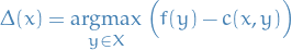
(notice it depends on
). Under the assumptions that  and that
  , we can equivalently consider

Classifier based on a separable cost function
 :=
\begin{cases}
\ \ \ 1 & \quad \text{if } c_i(x) \ge t \\
-1 & \quad \text{if } c_i(x) < t
\end{cases}
\end{equation*}](../../assets/latex/strategic_planning_4c5ee0bcc6a564c14245222d726a6ffe51a9a2bb.png)
for some
 .
.
Define the following
For classifier
, we define
which can also be expressed as
![$c_2[s]$](../../assets/latex/strategic_planning_d78e4531c48ba367edbb4fb1225f1de2b7d89d53.png) with
with 
Introduction
Model
Full-information game
The players are Jury and Contestant. Let
 be a fixed population
- a probability distribution over
 be a fixed cost function
 be the target classifier
Then a full information (2-player) game is defined as follows:
Jurypublishes a classifier
- cost function
- true classifier
- distribution
- cost function
Contestantproduces a function . The following information available to the
 Contestant:- cost function
Jury's classifier- true classifier
- distribution
- cost function
The payoffs are:
Jury:
Contestant:
- quantifies how much it costs for the
Contestantto change the input to theJury  is the change in the input made by the
 Contestant- Full information game is an example of a Stackelberg competition
- A Stackelberg competition is a game where the first player (
Jury) has the ability to commit to her strategy (a classifier) before the second player (Contestant) responds. - Wish to find a Stackelberg equilibrium, that is, a highest-payoff strategy for
Jury, assuming best response ofContestant- Equivalently, a perfect equilibrium in the corresponding strategic-form game
- A Stackelberg competition is a game where the first player (
The
Contestant knows the true classifier AND the Jury's classifier , while the Jury does not know the Contestant's function .
The Contestant knows the true classifier AND the Jury's classifier , while the Jury assumes Contestant chooses the optimal .
- Best outcome for
Juryis of course to find such that  for all
- Best outcome for
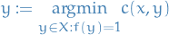
Contestantis to find s.t. is always classified as a "positive" example i.e. (assuming no cost)
In general, we'll simply have
which will then of course maximize the payoff for the
Contestant. This motivates the definition of the strategic maximum.
The strategic maximum in a full-information game is defined as
where is defined (as above)
(notice it depends on )
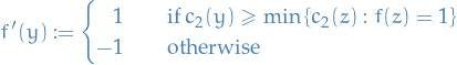
Suppose , i.e. zero-cost for Contestant to not move. Then we have the following characterization
- if
 , then
- We assuming that if one of the maximas defining is then we pick , rather than one of the other maximas
- We assuming that if one of the maximas defining
if
 , then we let
then
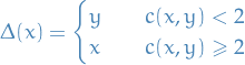
- Here we're just trying to find the "nearest" (in cost) point
 such that it will be classified as a positive example
 - It is clear that if
 , then
  and checking values on either side of this boundary it's clear
- Here we're just trying to find the "nearest" (in cost) point
Statistical classification game
- Now neither the
Jurynor theContestanthas knowledge of and , but instead the Jurycan request samples (hence "statistical" in the name)
The players are Jury and Contestant. Let
- be a fixed population
- a probability distribution over
- be a fixed cost function
- be the target classifier
A statistical classification game is then defined as follows:
Jurycan request labeled examples of the form with , and publishes a classifier . The following information is available to the Jury:- the cost function
- the cost function
Contestantproduces a function. The following information is available to the Contestant:- cost function
Jury's classifier
- cost function
The payoffs are:
Jury:
Contestant:![\begin{equation*}
\mathbb{E}_{x \sim \mathcal{D}} \big[ f \big( \Delta(x) \big) - c \big( x, \Delta(x) \big) \big]
\end{equation*}](../../assets/latex/strategic_planning_769bcbb23b5ea5b32cc111ffe7f9d3ab73950421.png)
Strategy-robust learning
Let be an algorithm producing a classifier .
If for
- all distributions
- for all classifiers
- for all
 (
( denoting the space of cost functions)
 - for all

given a description of and access to labeled examples of the form where , produces a classifier so that
![\begin{equation*}
\mathbb{P}_{x \sim \mathcal{D}} \big[ h(x) = f \big( \Delta(x) \big) \big] \ge \mathrm{OPT}_h(\mathcal{D}, c) - \varepsilon \quad \text{wp.} \quad 1 - \delta
\end{equation*}](../../assets/latex/strategic_planning_ae9c028e36ff485bda44b3f9872f35dba477bf7a.png)
where
Then we say that is a strategy-robust learning algorithm for .
One might expect, as with PAC-learning, that a strategy-robust learning algorithm might be restrict to be in some concept class  , however this will turn out not to be the case!
Separable cost functions
A cost function  is called separable if it can be written as

for functions  satisfying .
- The condition means that there is always a 0-cost option, i.e.
Contestantcan opt not to game and thus pay nothing- Since this means that
 s.t.
s.t. 
- Since this means that
For a class  of functions
  , the Rademacher complexity of with sample size
  is defined as
![\begin{equation*}
R_m(\mathcal{F}) := \mathbb{E}_{x_1, \dots, x_m \sim \mathcal{D}} \mathbb{E}_{\sigma_1, \dots, \sigma_m} \Bigg[ \sup_{f \in \mathcal{F}} \bigg( \frac{1}{m} \sum_{i=1}^{m} \sigma_i f(x_i) \bigg) \Bigg]
\end{equation*}](../../assets/latex/strategic_planning_68dcdcc02520352e684b381b72099f58944550e3.png)
where  are i.i.d. Rademacher random variables, i.e.
  .
.
Rademacher random variables can be considered as a "random classifier", and thus  kind of describes how well we can correlate the classifiers in with a random classifier.
 is the set of
  s.t. when is the best response of
 Contestant.
 : Let
: Let  .
.
- Suppose , then
 and we're done.
 Suppose
 , but that s.t.
  .
.

The question is then whether or not the argmax is outside or inside the 2-ball. If
 , we immediately have

i.e.
 since aims to maximize the above and returning is strictly a better option. Hence we must have
  s.t.
s.t.  , which is guaranteed to exists since we can just let
  .
.
Therefore, if then  , i.e.
  .
.
 : Let s.t. . Suppose, for the sake of contradiction, that
  . Then
  s.t.
s.t.  and
and  , because if such a existed we would have
  , contradicting the assumption that . Since, by assumption,
  for all
  , we must therefore have that
  , i.e. .
Note that

Hence
And to see that we can equivalently consider the classifier  , we can rewrite the
 Jury's payoff as

where
 is basically all
  such that and
  OR
OR  and
and  , i.e. all the mistakes
- Complement of the above is the all the correct classifications
Noting that if we did the same for , the only necessary change would be  :
:
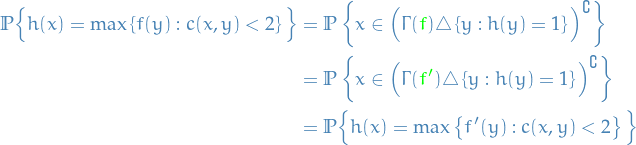
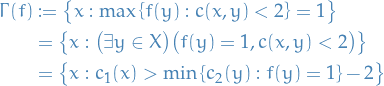
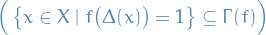
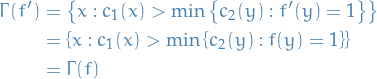
Note that
![\begin{equation*}
\Gamma(f) = \Gamma(f') = \Gamma(c_2[s]) = \left\{ x: c_1(x) > s - 2 \right\} = \big\{ x: c_1[s - 2](x) = 1 \big\}
\end{equation*}](../../assets/latex/strategic_planning_e87fe576515dfff9f2367882b05ffda1e7014539.png)
where

miller19_strat_class_is_causal_model_disguis
Notation
- Exogenous variables refer to variables whose value is determined outside the model and is imposed on the model
- Endogenous variables refer to variables whose value is determined by or inside the model.
 exogenous variables
 endogenous variables
In a structural causal model (SCM), a set of structural equations determine the values of the endogenous variables:

where
 represents the other endogenous variables that determine
  , and
, and  represents exogenous noise due to unmodeled factors
- An intervention is a modification to the structural equations of an SCM, e.g. an intervention may consist of replacing the structural equation
 with a new structural equation
  that holds at a fixed value
  denotes the variable
  in the modified SCM with structural equation
  , where and are two endogenous nodes of the SCM
 denotes the deterministic value of the endogenous variable when the exogenous variables are equal to
- Given some event
 , we denote
  the rv. in the modified SCM with structural equations where the distribution of the exogenous variables is updated by conditioning on the event ; this is what's referred to as a counterfactual
dong17_strat_class_from_reveal_prefer
Institution's utility (Stackelberg regret):
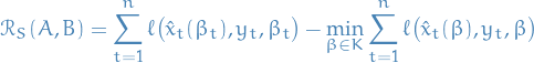
where
 denotes the loss function for the classifier
 denotes the sequence of agents
 denotes the sequence of classifier-parameters
Individual's utility:

- Each roundt :
- Institution commits to linear classifier parameterized by

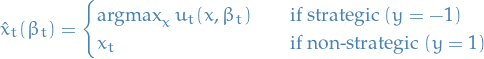
- An adversary, oblivious to the institution's choices up to round , selects an agent

- Agent
 sends the data point
  to the learner:
 , then the agent is strategic and sends the best response defined:
 , then the agent is non-strategic and sends the true features to the institution

In conclusion, the revealed feature
is defined
- Institution observes
 and experiences classification loss
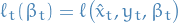
- Institution commits to linear classifier parameterized by
Assumptions:
- has bounded norm
 is convex, contains the
  and has norm bounded by
  , i.e.
  for all
Conditions for problem to be convex:
- Approach:
- Show that both choices of logistic and hinge loss for are convex if
 is convex.
- Show this under the case where
 for some satisfying some reasonable assumptions:
 is positive homogenouos of degree
  , i.e.

for any

- Show this under the case where
- Show that both choices of logistic and hinge loss for
Notation
 and
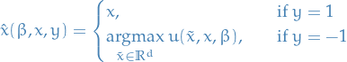
and  denotes the "manipulated" feature using the original feature . Assume manipulations occur only if "bad" label, i.e.
 and
and  represents the costs of the agent to change his features from to
  and
and  denotes the loss of the learner
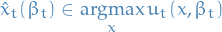
A strategic agent
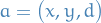 (with
(with  ), when facing a classifier
  , will misreport his feature vector as by solving the maximization problem
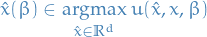
where the utility of the agent
 is defined

 denotes the subgradients of
 Stackelberg regret: for a history involving
 agents and the sequence of classifiers
  , the Stackelberg regret is defined to be
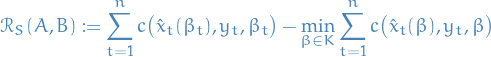
where
denotes the the optimal classifier (taking into account that the agents would behave differently)
In each strategic round, since
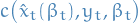
is a function of , we do not have direct access to the subgradients of and only see 0-th order information  . In this case we estimate the subgradient by minimizing a "smoothed" version of the classification loss: for any
  and parameter
  , the δ-smoothed version of is defined as flaxman04_onlin_convex_optim_bandit_settin
![\begin{equation*}
\overline{c}_t \big( \beta \big) := \mathbb{E} \big[ c_t \big( \beta + \delta S \big) \big]
\end{equation*}](../../assets/latex/strategic_planning_8a3f9cffa487aacbea6f810f477fd689792f289d.png)
where
 is a random vector drawn from the uniform distribution over
  .
.
Convex conjugate of a function
, denoted  is defined
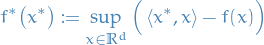
and is always convex
Main take-away
- Problem:
- Considers decisions through time (in contrast to hardt15_strat_class)
- Cost function is unknown to the learner
- Restricts the learner to linear classifiers
Agent's utility is then defined
- Similar to others:
- hardt15_strat_class: uses instead of and restricts the form of to be a separable
- haghtalab2020maximizing: uses mechanism instead of
- Though also restricts the mechanism to be, say, linear, in which case it becomes equivalent to the above
- hardt15_strat_class: uses
- Similar to others:
- Under sufficient conditions on the cost functions and agent cost
Strategic agent's best response set is
- Satisfied by examples:
Hinge loss:
Logistic loss:
- Focuses on obtaining conditions for when the cost function for the learner is convex
- Allows guarantees for neat cases, e.g. combination of strategic and non-strategic agents ("mixture feedback") by using convexity results from flaxman04_onlin_convex_optim_bandit_settin
- Drawbacks:
- No high-probability guarantees, but instead we just get bounds on the expectation of the Stackelberg regret
Conditions for a Convex Learning Problem
- This section describes the general conditions under which the learner's problem in our setting can be cast as a convex minimization problem
- Even if original loss function is convex wrt. (keeping and fixed), it may fail to be convex wrt. chosen strategically as a function of
- Even if original loss function is convex wrt.
4. Regret Minimization
4.1 Convex Optimization with Mixture Feedback
Let
 be the non-strategic rounds
 be the strategic rounds
Then for any
![\begin{equation*}
\mathbb{E} \Bigg[ \sum_{t=1}^{n} c_t \big( \beta_t^{ + } \big) - c_t(\beta) \Bigg] \le \mathbb{E} \Bigg[ \sum_{t \in T_{ - 1}}^{} \overline{c}_t(\beta) - \overline{c}_t(\beta) \Bigg] + \mathbb{E} \Bigg[ \sum_{t \in T_1}^{} c_t(\beta_t) - c_t(\beta) \Bigg] + 3 n L \delta
\end{equation*}](../../assets/latex/strategic_planning_faec6ccc27ce1e9b8953c7d772b3c90747e88f7c.png)
where the expectation is wrt. the randomness of the algorithm.
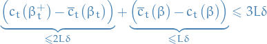
which implies

References
Bibliography
- [milli18_social_cost_strat_class] Milli, Miller, Dragan, & Hardt, The Social Cost of Strategic Classification, CoRR, (2018). link.
- [rambachan2020economic] Rambachan, Kleinberg, Mullainathan & Ludwig, An Economic Approach to Regulating Algorithms, , (2020).
- [dong17_strat_class_from_reveal_prefer] Dong, Roth, Schutzman, , Waggoner & Wu, Strategic Classification From Revealed Preferences, CoRR, (2017). link.
- [nesterov2017random] Nesterov & Spokoiny, Random gradient-free minimization of convex functions, Foundations of Computational Mathematics, 17(2), 527-566 (2017).
- [hardt15_strat_class] Hardt, Megiddo, Papadimitriou, Christos & Wootters, Strategic Classification, CoRR, (2015). link.
- [hu18_dispar_effec_strat_manip] Hu, Immorlica, Vaughan & Wortman, The Disparate Effects of Strategic Manipulation, CoRR, (2018). link.
- [roth15_watch_learn] Roth, Ullman, Wu & Steven, Watch and Learn: Optimizing From Revealed Preferences Feedback, CoRR, (2015). link.
- [miller19_strat_class_is_causal_model_disguis] Miller, Milli & Hardt, Strategic Classification Is Causal Modeling in Disguise, CoRR, (2019). link.
- [haghtalab2020maximizing] Haghtalab, Immorlica, Lucier & Wang, Maximizing Welfare with Incentive-Aware Evaluation Mechanisms, , (2020).
- [flaxman04_onlin_convex_optim_bandit_settin] Flaxman, Kalai, & McMahan, Online Convex Optimization in the Bandit Setting: Gradient Descent Without a Gradient, CoRR, (2004). link.
- [perdomo20_perfor_predic] Perdomo, Zrnic, , Mendler-D\"unner & Hardt, Performative Prediction, CoRR, (2020). link.
- [liu19_dispar_equil_algor_decis_makin] Liu, Wilson, Haghtalab, , Kalai, Borgs, & Chayes, The Disparate Equilibria of Algorithmic Decision Making When Individuals Invest Rationally, CoRR, (2019). link.
- [frazier2014incentivizing] Frazier, Kempe, Kleinberg & Kleinberg, Incentivizing exploration, 5-22, in in: Proceedings of the fifteenth ACM conference on Economics and computation, edited by (2014)
- [zinkevich2003online] Zinkevich, Online convex programming and generalized infinitesimal gradient ascent, 928-936, in in: Proceedings of the 20th international conference on machine learning (icml-03), edited by (2003)