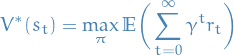
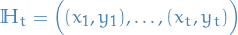
Reinforcement Learning
Table of Contents
Overview
Reinforcement Learning is a learning framework where which helps us to account for
future reward by "encoding" the value of the next state  (and / or actions)
in the value of the current state
(and / or actions)
in the value of the current state  (and / or actions), thus turning the
greedy "strategy", wrt. this value function we're creating, the optimal "strategy".
(and / or actions), thus turning the
greedy "strategy", wrt. this value function we're creating, the optimal "strategy".
Notation
- Capital letter = random variable, e.g.
 is the random variable which can take on all
- Wierd capital letters = spaces of values that the random variables can take on, e.g. reward space / function

- Lowercase = specific values the random variables take on, e.g.
![$\mathbb{E}[S = s]$](../../assets/latex/reinforcement_learning_53205038419d901a8e4b075f96927a0a0254be52.png)
 denotes optimality for some function
 - policy
 - action
- - state
 - reward
 - value function for some state
 - accumulated reward at step
Markov Decision Process
Markov Reward Process (MRP)
See p. 10 in the Lecture 2: MDP.
Markov Decision Process (MDP)
See p. 24 in the Lecture 2: MDP.
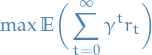
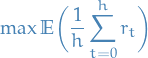
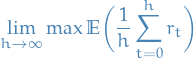
Optimality in MDP
 , i.e. the problem is now
![\begin{equation*}
\max \mathbb{E} \bigg[ \sum_{t = 0}^{h} r_t \bigg]
\end{equation*}](../../assets/latex/reinforcement_learning_b918c5eed7451751cb30597601a18111f2cc24ed.png)
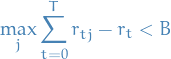
Learning performance
Asymptotic convergence

PAC learning:

for some
 .
.
Regret bound
for some
 .
.
- Assumes oracle
 exists
 - Regret doesn't tell you anything about each of the individual regrets

- Assumes oracle
Partial Observable Markov Decision Process (POMDP)
See p. 51 in the Lecture 2: MDP.
Planning by Dynamic Programming
Optimal state-value function:
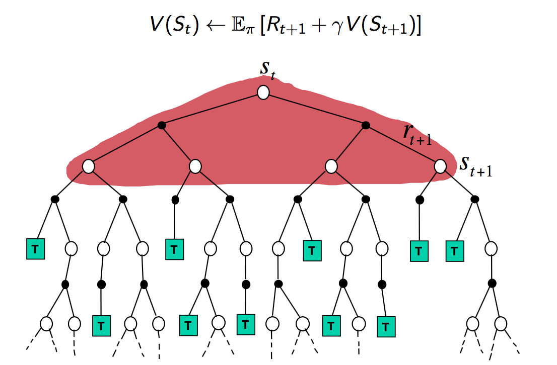
The Bellman equation defines recursively:

and then the Bellman optimality equation
Policy evaluation
Problem - evaluate a given policy
Solution - iterative application of Bellman expectation backup
- Initial value function
 is 0 everywhere
 - Using synchronous backups
- Each iteration

- For all states

- Update
 from
from 
- Each iteration
In short, when updating the value function  for state , we use the Bellman equation and the previous value function
  for all "neighboring" states (the states we can end up it with all the actions we can take).
 refers to the
  iteration of the iterative policy evaluation
Policy iteration
Problem: given a policy , find a better policy
- Evaluate the polciy
Improve the policy by acting greedily wrt. to
 ,
,
This will eventually converge to the optimal policy  due to the partial ordering of policies
  .
.
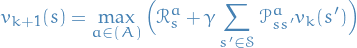
Value iteration
Problem
Find optimal policy given the dynamics of the systems (rewards and environmental state)
Solution
Iterative application of Bellman optimality backup.
- Initialize value function
- For each iteration

- For all states
- Update
 from
from 
- For all states
Unlike policy iteration, there is no explicity policy here.
At each iteration, for all states we make the current
optimal action  (i.e. optimal wrt. the current iteration),
and then update the value
(i.e. optimal wrt. the current iteration),
and then update the value  for this state.
Eventually  will converge to the true value function for some ,
and since all states are dependent through the recursive relationship from
the Bellman equation, the other states will also start to converge.
will converge to the true value function for some ,
and since all states are dependent through the recursive relationship from
the Bellman equation, the other states will also start to converge.
In the form of the Bellman equation we can write the iterative process as:
 1
1
Or in matrix notation:
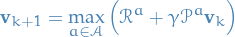 2
2
Summary
| Problem | Bellman equation | Algorithm |
|---|---|---|
| Prediction | Bellman Expectation equation | Iterative, Policy evaluation |
| Control (maximize reward) | Bellman Expectation equation + Greedy Policy improvement | Policy iteration |
| Control | Bellman Optimality equation | Value iteration |
Extensions
Asynchronous Dynamic Programming
Prioritized sweeping
- Decide which states to update
- Use absolute value between Bellman equation update and current to
guide our selection for which states to update
Real-time dynamic programming
- Idea: only the states that are relevant to agent
- Randomly sample
- After each time-step

- Backup the state
Model-free Prediction - policy-evaluation
What if we don't know the Markov Decision Process, i.e. how the environment works?
This sections focuses only on evaluating the value function  for some given
policy . This policy does not have to be the optimal policy. ONE STEP AT THE TIME
BOIS!
for some given
policy . This policy does not have to be the optimal policy. ONE STEP AT THE TIME
BOIS!
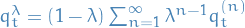
Monte-Carlo Learning
Notation
 - # of times we've seen state in this episode
 - sum of values received from the times we've been in state
in this episode
- sum of values received from the times we've been in state
in this episode
Overview
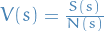
valueis equal toavg. return- Learns from complete episodes, i.e. we need to reach some termination
- Caveat can only apply MC to episodic
We assume ![$v_\pi = \mathbb{E} [G_t | S_t = s]$](../../assets/latex/reinforcement_learning_65c54f712d20e3e7d0ed2e42f609c1acb81c23b7.png) , and so all we try to do is find the avg.
accumulated reward starting from our current state at step .
, and so all we try to do is find the avg.
accumulated reward starting from our current state at step .
To obtain this average, we sample "mini-episodes" starting from our current state
and average the accumulated reward  over these samples.
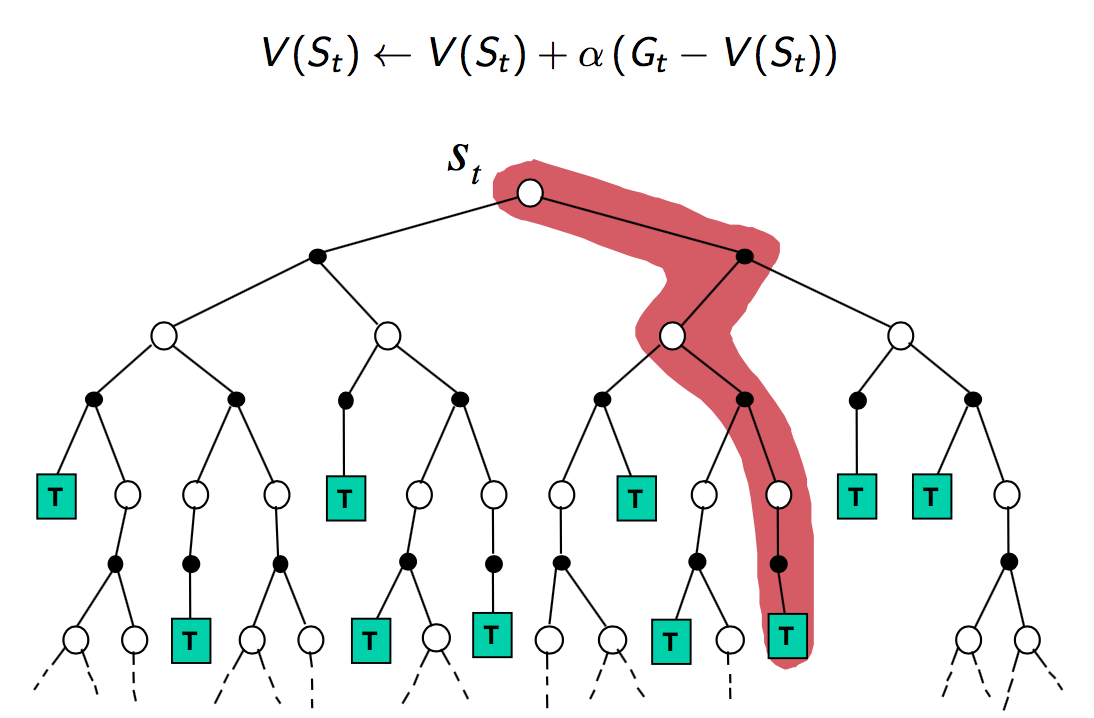
First-Visit MC policy evaluation
The first time-step in that state is visited in an (sampled) episode:
- Increment counter
- Increment total return
 , ( being the sum in this case)
 - Value is estimated by mean return
- By law of large numbers,

Instead of using the total sums, we can take advantage of the recursive mean formula for online-learning.
Every-Visit MC policy evaluation
Same as First-Visit MC policy evaluation, but if we have loops and end up in the
same state multiple times in the same episode, we perform the steps above.
Incremental MC
See p. 11 in Lecture 4.
Update is now:
 3
3
where  in this case. The above is basically a general approach
which we will see recurring in other methods.
in this case. The above is basically a general approach
which we will see recurring in other methods.
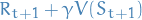
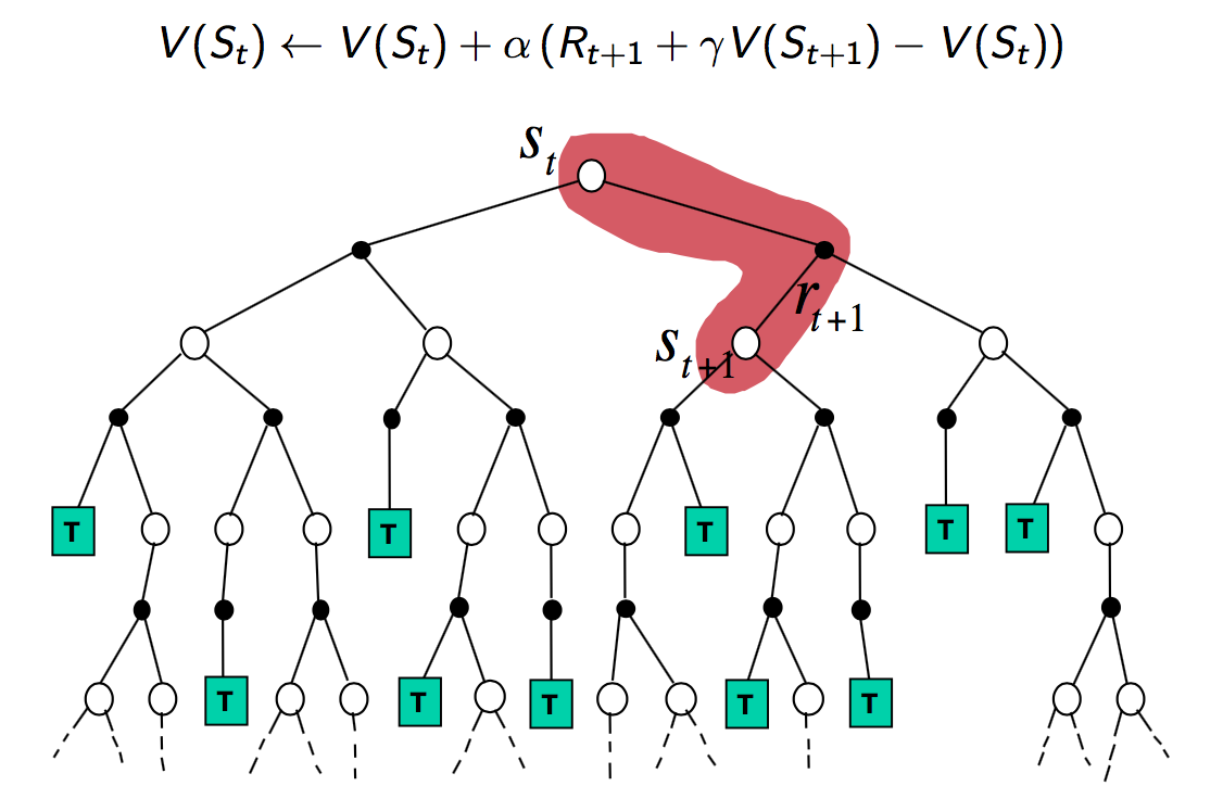
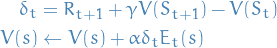
Temporal-Difference Learning
Notation
- TD-target -
 , i.e. the value of state we
we want to update towards. Thus we update
, i.e. the value of state we
we want to update towards. Thus we update  to better account for the
value of the next state.
to better account for the
value of the next state. - TD-error -
 , i.e.
Overview
- Learn directly from experience
- No knowledge of MDP transitions / rewards, i.e. model-free
- Learns from incomplete episodes, by bootstrapping (different from MC)
- Updates a guess towards a guess
- TD attempts to "encode" a fraction of the value in the next state
into the value of incrementally
Update value towards estimated return
 4
4
- TD-target
- TD-error
The difference between the MC and TD approaches is that the MC considers the
actual return obtained from an (complete) episode, while the TD
uses some estimated return at the next step to obtain value for current step.
TD is thus a much more flexible approach than MC.
Check out p.15 in Lecture 4 for a really nice example of the difference!
Bias / Variance between MC and TD
- Return
 is unbiased
estimate of
is unbiased
estimate of 
- If we had the true value function, TD would also be unbiased, BUT it ain't so!
- TD target is biased estimate of ,
but has lower variance
- MC's evaluation depends on many random actions, transitions, rewards
- TD's evaluation depends only on one random action, transition, reward
Pros and cons
- MC has high variance, zerio bias
- Good convergence properties
- (also for function-approximations)
- Not very sensitive to initial value
- Minimizes the mean-squared error (p. 24 Lecture 4)
- Ignores the Markov property
- Slower when Markov property is present
- Works even though there is no Markov property
- Uses sampling
- Good convergence properties
- TD has low variance, some bias
- Usually more efficient than MC
- TD(0) converges to

- (not always for function-approximations)
- More sensitive to initial value
- Converges to a solution of maximum likelihood Markov model (p. 24 Lecture 4)
- Takes advantage of the Markov property
- Faster when this is present
- Does not work as well when Markov property is absent
- Usues bootstrapping AND sampling
DO checkout p. 26-28 in Lecture 4! It shows some great visualizations of the different methods and how they do look-aheads / backups.
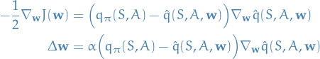
TD(λ)
- Sweet-spot between TD- and MC-learning
- What if we instead of just considering the very next reward,
we consider the
 next rewards!
 - But we would also like to more heavily weight the more immediate reward
estimates, compared to one found steps into the future.
Let's define the n-step return as :
 5
5
The update is then:
 6
6
And we get, as Hannah Montana would say, the best of both worlds! (TM)
The issue now is to find the optimal .
To handle this, we would like to somehow take the average reward for the different
. And so TD(λ) is born!
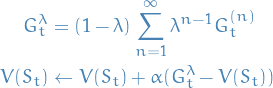
Forward-view TD(λ)
- The λ-return
 combines all n-step returns
Using weight

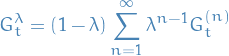 7
7
Forward-view TD(λ)
 8
8
- Why geometric weighting, and not some other weighting?
- Computationally efficient
- Stateless => no more expensive than TD(0)
- Issue is now that we have to wait until the end of the episode (since we're summing
to infinity), which is the same problem we had with MC
- Luckily, by taking on an additional view of the problem, backward-view TD(λ), we can update from incomplete episodes
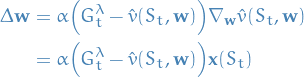
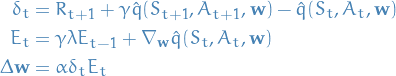
Backward-view TD(λ)
- Keep eligibility trace for every state
- Update value for
 for every state
 Update happens in proportion to the TD-error
 and the eligibility-trace
 9
9
Eligibility traces
Eligibility traces combines most frequent and most recent states:
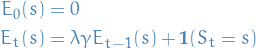 10
10
My intuition regarding this is as follows:
- Gives us a way of measuring "responsibility" for the TD-error
- If we at some time-step
 end up in state , then at some
we end up in the same state , we can view the
eligibility trace of at
end up in state , then at some
we end up in the same state , we can view the
eligibility trace of at  to measure how much the
error in the value function is due to what we saw steps back.
to measure how much the
error in the value function is due to what we saw steps back.
See p.40 in Lecture 4 for an example.
Replacing Eligibility Trace method
The concept is simple; instead of adding the weighted occurence to the trace, we simply replace it. This way the largest possible contribution we can have is 1.
This is especially useful for cases where we have possibilities of cyclic state-transitions, as the multiple occurences of the same state can lead to incredibly contributions to this state.
Take this example:
- Start at position 0
- Reward is at position 1
- Try to move left (opposite of reward) 100000 times, staying in position 0 since there is a wall to our left
- Finally take a right
- Receive reward
In this case position 0 would get large amounts of credit even though it might not be the best state to be in.
This can also often lead to integer-overflow unless other precautionary measures are taken.
For completeness:
![\begin{equation*}
E_t[s, a] \leftarrow 1
\end{equation*}](../../assets/latex/reinforcement_learning_5844c77d330bf5f70344cbd29e39e605c483d1cd.png) 11
11
is used instead of
![\begin{equation*}
E_t[s, a] \leftarrow E_{t-1}[s, a] + 1
\end{equation*}](../../assets/latex/reinforcement_learning_a236271dda09ffaa552d536e67e278f683366391.png) 12
12
Backward-view and forward-view equivalence
If you have a look at p.43 in Lecture 4 and on, there is some stuff about the fact that these views are equivalent.
TD(0) is simply the Simple TD-learning we started out with:
 13
13
TD(1) defers updates until the episode has terminated:
 14
14
This is not actually equivalent to the MC view, just sayin'.
Conclusion
Forward-view provides us with a "theoretical", providing us with an intuition
 15
15
Backward-view provides us with a practical way to update
for
some state where the error is now a function of the previous
updates of instead of the future updates, as in the forward view.
16
- Backward-view provides us with a practical way to update some state
a any time-step by saying that this state depends on a combined
weight of the steps since we last updated and the frequency of
state . If we let
 , i.e. consider
  , it turns out that
the forward-view and backward-view are equivalent.
, it turns out that
the forward-view and backward-view are equivalent.
I must admit that I'm sort of having a hard time understanding how the forward-view and backward-view are in fact equivalent.
I can understand the intuition behind both views, but it does not seem to be the same intuition. Forward-view:
- TD-error is difference between current and accumulated rewards
at all steps in the future
Backward-view:
- Considers all previous updates to for the state
Both:
- The error between
 now and in some future is of course zero if
we never actually see state again. This also makes sense in the backward-view,
where at some "future" we haven't seen since some time in the past.
now and in some future is of course zero if
we never actually see state again. This also makes sense in the backward-view,
where at some "future" we haven't seen since some time in the past.
Model-free Control - policy-optimization
On-policy
Sarsa
- Uses TD-learning to learn

- Updates to
Sarsa(λ)
Sarsa(1)
- Elegibility trace runs all the way back => how do we deal with loops?
- Cycles of identical state-action pair
 will cause updates
which lowers
will cause updates
which lowers  until it is not any longer the preferred pair.
 - But what if is in fact the best state-action pair, but also
has the largest probability of ending up in , then the above point
would be highly indesirable!
- This is especially a problem in environemnts where we dont get a reward until the episode terminates
- In this case, lowering the eligility-factor (or whatever you call it)
 might help to mitigate this (I think o.O)
- Cycles of identical state-action pair
Off-policy
Q-Learning
Attempts to estimate a target policy
 and use this to then estimate or

Notice the difference between Sarsa and Q-learning!
 is observed,
  is predicted from
Properties
- Probably converge in infinite-data limit, assuming every state is visited infintely often
- In the tabular context, Q-learning is provably sample efficient jin18_is_q_learn_provab_effic
Value-function approximation
Incremental methods
Value function approximation
Monte-Carlo
TD
TD(λ)
- λ-return is a biased sample of true value
Apply supervised learning to "training data"

 is now be of same dimension as our feature-space!
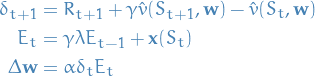
Action-value function approximation
Evaluation / prediction
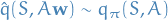
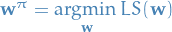
Want to minimise the mean-squared error (MSE):
![\begin{equation*}
\underset{\mathbf{w}}{\text{argmin }} \mathbb{E}_\pi \Big[ \Big( q_\pi (S, A) - \hat{q} (S, A, \mathbf{w}) \Big)^2 \Big]
\end{equation*}](../../assets/latex/reinforcement_learning_586c661db8d265ebdecc07df1440007cc0f8f0dc.png)
Using SGD to find local minimum:
Control
Simply take what we found in Evaluation / prediction and substitute
a target for 


 , thus:

 and
and  .
.
Batch methods
Thought is to "re-use" data, or rather, make the most use of the data we have, instead of updating once using each point as previously described.
Experience replay
See p.35 in Lecture 6.
But it's basically just this:
- Sample
 from our observations
- Apply SGD update
- Converges to least squares solution
Deep Q-Networks (DQN)
See p.40 or so in Lecture 6 for this awesomesauce. Uses
- Experience replay
- Randomization decorrelates the data => good!
- Fixed Q-targets
- Freeze network, and then during the next training-cycle we bootstrap towards the frozen network (just old parameters)
- Every some
nsteps we freeze the parameters, and then the nextnsteps we use these parameters' prediction as targets. Then after thosentargets we freeze our new parameters, and repeat. - More stable update
The points above is what makes this non-linear function approx. stable.
What they did in the Atari-paper is to have the outputs of the
ConvNet be a softmax over all possible actions. This allows
easy maximization over the actions, and is not too hard to model
as long as the action-space  isn't too large.
Linear Least Squares prediction
See p. 43 or so for a closed form solution to the linear case. For prediction, but something similar exists for control too.
Policy gradient methods
Notation
 is any policy objective function
 is the policy update
Introduction
Previously we've considered the prediction and control of the value function, but now we're instead going to directly model the optimal policy! That is, we directly parametrise
![\begin{equation*}
\pi_\theta = \mathcal{P} [a, | s, \theta]
\end{equation*}](../../assets/latex/reinforcement_learning_d9126a8151880d3d2617c4da841a3074d8a86afd.png) 17
17
To be able to optimize the policy, we first need to come up with some policy objective function.
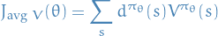
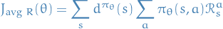
Policy Object Functions
Goal: given a policy  with parameters
  ,
find best
,
find best
Need to measure quality of  :
:
Episodic environment with some initial state, we use the start-value:
![\begin{equation*}
J_1 (\theta) = V^{\pi_\theta} (s_1) = \mathbb{E_{\pi_\theta}}[v_1]
\end{equation*}](../../assets/latex/reinforcement_learning_d65a1cbe9f88f5836bb49df88d7bc7a1c6ee50a3.png) 18
18
i.e. judge the policy by the expected reward received when starting in state

Continuing environments we can use the average value:
 19
19
Or average reward per time-step
 20
20
which says "there is some probability of being in state
, under our
policy there is some probability I choose action in this state,
and then I receive reward at this step". So the above is for each time-step.
Where
 is a stationary distribution of a Markov Chain, i.e.
what is the probability of being in state .
is a stationary distribution of a Markov Chain, i.e.
what is the probability of being in state .
Comparison with Value-based methods
Advantages
- Better convergence propertiers
- Effective in high-dimensional or continuous action space
- This is due to the fact that in value-based methods we need to maximize over the actions to obtain the "value" for a next state. With high-dimensional or continuous action space it might be very hard to perform this maximization
- Can learn stochastic policies
- stochastic policies simply mean policies which take on a probability distribution over the actions rather than a discrete choice. Very useful when the environment itself is stochastic (i.e. not deterministic).
- Example is "Rock-Paper-Scissor", where a the optimal behavior will be a uniform distribution over the actions.
Disadvantages
- Typically converge to local optimum rather than global
- Policy evaluation is usually inefficient using Policy Gradient Methods, compared to using Value-function methods.
Finite Difference Policy Gradient
- To evaluate policy gradient of
- Does so through the definition of the derivative for each dimension (see p. 13 in Lecture 7 for details)
- Noisy and inefficent in high dimensions
Monte-Carlo Policy Gradient
- Allows analytic gradients
- Assume policy is differnetiable whenever it is non-zero
- And know the gradient
Score function:
 21
21
where we simply ignore the
term from the Likelihood ratios
due to the fact that optimizing wrt.  also optimizes
  .
.
Likelihood ratios
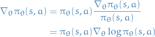 22
22
Simply due to the 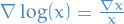
Example score-function: Softmax Policy
- Actions weighted by linear combination of features

- Assume
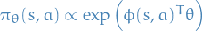
Score function is then
![\begin{equation*}
\nabla_\theta \log \pi_\theta (s, a) = \phi(s, a) - \mathbb{E} [\phi(s, \cdot)]
\end{equation*}](../../assets/latex/reinforcement_learning_7859bf7d12cb33a5fc6a57347ab04c12f0847743.png) 23
23
Example score-function: Gaussian Policy
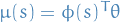
- Policy is Guassian,
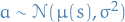
Score function is then
 24
24
One-Step MDPs
- Starting in state

- Terminating after one time-step with reward

See p. 19 in Lecture 7 for how to compute the policy gradient, OR try it yourself from the objective functions described earlier!
![\begin{equation*}
\nabla_\theta J(\theta) = \mathbb{E}_{\pi_\theta} [\nabla_\theta \log \pi_\theta (s, a) r]
\end{equation*}](../../assets/latex/reinforcement_learning_6cb640a76e12c548081431c25f9e9198bb441b2e.png) 25
25
Policy Gradient Theorem
Simply changes the immediate reward  in the one-step MDPs with
the long-term value
in the one-step MDPs with
the long-term value  .
.
For any differentiable policy  ,
for any of the policy objective functions
,
for any of the policy objective functions  ,
the policy gradient is
,
the policy gradient is
![\begin{equation*}
\nabla_\theta J(\theta) = \mathbb{E}_{\pi_\theta} [\nabla_\theta \log \pi_\theta (s, a) Q^{\pi_\theta}(s, a)]
\end{equation*}](../../assets/latex/reinforcement_learning_0bcc1268302a28c372fb88d3faa0b61b7af90720.png) 26
26
The algorithm
- Update parameters by SGD
- Using policy gradient theorem
Using return
 as an unbiased sample of
 27
27
Remember this is a MC => need to sample entire episode to learn
See p.21 from Lecture 7 for psuedo-code.
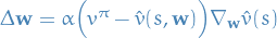
Actor-Critic Policy Gradient
- Actor-Critic learns both value function and policy
- MC policy gradient still has high variance
- Use critic to estimate the action-value function
- Actor-critic algorithms maintain two sets of parameters
- Critic
- updates action-value function parameters

- Actor
- updates policy parameters in direction suggested by critic
That is; critic handles estimating
 , and the actor then asks
the critic what the value of the state-action pair the critic just observed / took
is, and updates the policy-parameters according to this value
, and the actor then asks
the critic what the value of the state-action pair the critic just observed / took
is, and updates the policy-parameters according to this value
![\begin{equation*}
\begin{split}
\nabla_\theta J(\theta) &\sim \mathbb{E}_{\pi_\theta} [\nabla_\theta \log \pi_\theta (s, a) Q_w (s, a) ] \\
\Delta \theta &= \alpha \nabla_\theta \log \pi_\theta (s, a) Q_w(s, a)
\end{split}
\end{equation*}](../../assets/latex/reinforcement_learning_f1ebeec6ea6c3c6efdba5e9b4af87a9e89308b5c.png) 28
28
So we have exactly the same update, but now replacing the long-term action-value function with an approximation.
Estimating the action-value function
Want to know how good the current policy is for current params ,
hence we need to do policy evaluation
- Monte-Carlo policy evaluation
- Temporal-Difference evaluation
- TD(λ)
Algorithm
See the psuedo-code on p. 25 in Lecture 7.
But sort of what it does is (at each step):
- (actor) Sample
 ; sample transition
- (actor) Sample action
- (critic) Compute TD-error
- (actor) Update policy-parameters
- (critic) Update weights for

- (actor)

Compatible Function Approximation
If the following two conditions are satifisfied:
Value function approximator is compatible to the policy
 29
29
Value function parameters
minimise the MSE
![\begin{equation*}
\varepsilon = \mathbb{E} \Big[ \big( Q^{\pi_\theta}(s, a) - Q_w(s, a) \big)^2 \Big]
\end{equation*}](../../assets/latex/reinforcement_learning_f17481a2502dc1ba220ecb9132971cdac95d9c80.png) 30
30
Then the policy gradient is exact,
![\begin{equation*}
\nabla_\theta J(\theta) = \mathbb{E} \big[ \nabla_\theta \log \pi_\theta (s, a) Q_w(s,a) \big]
\end{equation*}](../../assets/latex/reinforcement_learning_1f711122baca544c82e669128ccbbd90da024383.png) 31
31
Reducing variance using a Baseline
- Subtract a baseline function
 from the policy gradient
 - Can reduce variance without changing expectation
- Basically "centering" (subtracting mean and dividing by variance)
See p. 30 in Lecture 7 for a proof of why it doesn't change the
expectation. Basically, we can add or subtract anything we want
from as long as it only depends on the state .
Left with something called the advantage function
![\begin{equation*}
\begin{split}
A^{\pi_\theta} (s, a) &= Q^{\pi_\theta} (s, a) - V^{\pi_\theta}(s) \\
\nabla_\theta J(\theta) &= \mathbb{E}_{\pi_\theta}[\nabla_\theta \log \pi_\theta (s, a) A^{\pi_\theta} (s, a)] \\
\end{split}
\end{equation*}](../../assets/latex/reinforcement_learning_2aa3df42d51bba609c70e35bba74c3eb2cb66f2e.png) 32
32
Estimating Advantage function
There multiple ways of doing this.
See p. 30 in Lecture 7 and on for some ways. The most used one is nr. 2.
Summary
Policy gradient has many equivalent forms:
![\begin{eqnarray*}
\nabla_\theta J(\theta) &=& \mathbb{E} [ \nabla_\theta \log \pi_\theta (s, a) v(s)] & \text{REINFORCE} \\
&=& \mathbb{E} [ \nabla_\theta \log \pi_\theta (s, a) Q^w (s, a) ] & \text{Q Actor-Critic} \\
&=& \mathbb{E} [ \nabla_\theta \log \pi_\theta (s, a) A^{\pi_\theta}(s, a) ] & \text{Advantage Actor-Critic} \\
&=& \mathbb{E} [ \nabla_\theta \log \pi_\theta (s, a) \delta ] & \text{TD Actor-Critic} \\
&=& \mathbb{E} [ \nabla_\theta \log \pi_\theta (s, a) \delta e ] & \text{TD(}\lambda \text{) Actor-Critic} \\
G_\theta^{-1} \nabla_\theta J(\theta) &=& w & \text{Natural Actor-Critic}
\end{eqnarray*}](../../assets/latex/reinforcement_learning_5ebbc0f67489b89da8c390a941bbc52471c0cb50.png) 33
33
All these methods are basically saying: move the policy in the direction that gets us more value.
- Each leads a SGD algorithm
- Critic uses policy evaluation (e.g. MC or TD learning) to estimate
 ,
,
 or
or 
Thompson sampling
Notation
 actions
 are the probabilities of success for the corresponding action / arm
 denotes a graph with vertices
  and edges
Historical data
 denotes reward obtained by taking action
  leading to observed outcome
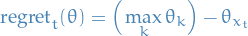
Per-period regret is the difference between exptected reward using optimal action and the reward received by current action. In the Armed bandit problem:
 is the conditional distribution of the system (i.e. what we want to learn)
Armed bandit
- Suppose there are
 actions, and when played, any action yields either a success or failure.
 - Action produces a success with probability
![$\theta_k \in [0, 1]$](../../assets/latex/reinforcement_learning_29346ae1bdf6bd2b871a035b1ceb55a9966b1075.png) .
. - The success probabilities are unknown to the agent, but are fixed over time, and can therefore be learned by experimentation
- Objective: maximize number of successes over
 periods, where is relatively large compared to the number of arms
Stuff
- Posterior sampling and probability matching
- Methods such as
 attempts to balance exploration by choosing a random action with probability
  and greedy step with probability
- Inefficient since it will sample actions regardless of how unlikely they are to be optimal; Thompson sampling attempts to address this
- Useful for online decision problems
![\begin{algorithm*}[H]
\KwData{action space $\mathcal{X}$, prior $p$, enviroment distribution $q$, reward function $r$}
\KwResult{posterior distribution $\hat{p}$}
\For{$t = 1, 2, \dots$} {
\tcp{sample model; a greedy algorithm would use $\hat{\theta} = \mathbb{E}_p[\theta]$}
$\hat{\theta} \sim p$ \\
\tcp{select and apply action}
$x_t \leftarrow \underset{x \in \mathcal{X}}{\text{argmax}}\ \mathbb{E}_{q_{\hat{\theta}}} \big[ r(y_t) \mid x_t = x \big]$ \\
Apply $x_t$ and observe $y_t$ \\
\tcp{update distribution}
$p \leftarrow \mathbb{P}_{p, q}(\theta \in \cdot \mid x_t, y_t)$
}
\caption{Thompson Sampling. Estimate the distribution of the environment. }
\end{algorithm*}](../../assets/latex/reinforcement_learning_cb4cd1ba5733728e974fc6b58fe2af5926da3cb1.png) 34
34
The difference between a greedy algorithm and Thompson sampling is that a greedy algorithm would use the expectation over the current estimate of  to obtain the new estimate of , while Thompson sampling samples the new estimate of .
Book
Chapter 2
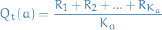
Stationary Problem
- N-armed bandit problem
- Action-rewards does not change over time but stay constant
- All we got to do then is to model the average reward for some action, i.e.
 34
34
where  is the number times we've chosen action up until step
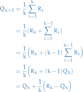
And of course, practically it's better to compute this using the recursive formula for the mean:
 35
35
where  is the value for some action after choosing
and receiving reward from this action
is the value for some action after choosing
and receiving reward from this action  times.
Non-stationary Problem
- Makes sense to more heavily weight the most recent observations higher than "old" ones
- We write
 in instead of
  to be a bit more general
 - By recursively expanding we obtain
 36
36
Which is called the weighted average, due to the fact that
 (can be proven by induction).
Exercises
2.3 - N-Armed bandit ɛ-greedy comparison
Consider the following learning problem. You are faced repeatedly with a choice among
n different options, or actions. After each choice you receive a numerical reward
chosen from a stationary probability distribution that depends on the action you selected.
Your objective is to maximize the expected total reward over some time period,
for example, over 1000 action selections,or time steps.
The problem is as follows:
- Choose between
nactions at each stept - Action-rewards are constant wrt.
t - Maximize expected / avg. reward over 1000 steps
t
To get an idea of how well the algorithms perform in general, we run the above for 2000 different action-rewards, i.e. 2000 differently parametrized environments.
# don't want this tangled
%matplotlib inline
import numpy as np
import matplotlib.pyplot as plt

# n-Armed Bandit
# each environment has 10 actions (bandits), and we have 2000 such problems
# allows us to see how algorithms perform over different hidden action-values
n_steps = 1000
n_problems = 2000
armed_testbed = np.random.randn(10, n_problems)
actions = np.arange(10)
steps = np.arange(n_steps)

# we compute the value of action `a` at step `t`
# by the accumulated reward from the times we've
# chosen `a` up until (incl.) `t` and then divided
# by the number of times we've chosen this `a`.
# Basically, the average reward of `a` at `t`
# wrt. times we've chosen `a`.


def epsilon_greedy(Q, epsilon):
    if np.random.rand() < epsilon:
        return np.random.randint(actions.shape[0])
    return np.argmax(Q)


def run_testbed(choose_action, *args, **kwargs):
    rewards = np.zeros((n_steps, armed_testbed.shape[1]))

    for j in range(armed_testbed.shape[1]):
        environment = armed_testbed[:, j]

        # intialization
        Q = np.zeros(10)
        action_freq = np.zeros_like(actions, dtype=np.int)
        action_reward = np.zeros_like(actions)
        reward = 0

        for t in steps:
            a = choose_action(Q, *args, **kwargs)
            # reward with some noise
            r = environment[a] + np.random.randn()
            # update count and reward for selection action `a`
            action_freq[a] += 1
            action_reward[a] += r
            # update value for action `a`
            Q = action_reward / (action_freq + 1e-5)

            # accumulate reward
            reward += r
            # expected reward wrt. t
            rewards[t, j] = reward / (t or 1)

    # take the avg for each time-step over all problems
    return np.mean(rewards, axis=1)
And let's run the testbed for different ε in parallel.
import multiprocessing as mp
from functools import partial

f = partial(run_testbed, epsilon_greedy)

with mp.Pool(3) as p:
    results = p.map(f, [0, 0.01, 0.1])
Finally we create the plot!
steps = np.arange(1000)

fig = plt.figure(figsize=(14, 5))
plt.plot(steps, results[0], label="greedy")
plt.plot(steps, results[1], label="ε-greedy 0.01")
plt.plot(steps, results[2], label="ε-greedy 0.1")
plt.title("2000 different 10-bandit problems")
plt.ylabel("Expected $R_t$")
plt.xlabel("$t$")
plt.legend()
plt.show()
Defintions
- synchronous updates
- update all states / values / whatever one after the other
- prediction
- given a full MDP and some policy , find value function
 for this policy
 - control
- given a full MDP, find optimal (wrt. reward) value function
 and policy
- backup
- simply the state we "base" our update on for some state

- backup
- updating the value of a state using values of future states
- full backup
- we perform backup for all states
- sweep
- consists of applying a backup operation to each state
- TD-target
- TD-error
- bootstrapping
- update involves an estimate (not the real returns / rewards)
- sampling
- update samples an expectation
- stochastic policy
- policy which uses a distribution over actions rather than deterministic behavior.
Resources
- Karpathy's "Pong from pixels". Details how to implement a policy-gradient RL-algorithm using a ConvNet for function-approximation to learn to play Pong from the raw image input.