PyTorch
Table of Contents
Overview
- Tensor computation (like numpy) with strong GPU acceleration
- Deep Neural Networks built on tape-based autograd system
- Tape-based autograd = keeps track of computation you perform with variables
- Allows for dynamic neural networks, i.e. change the way the net works arbitrarily with zero lag or overhead
If you ever want a nice introduction, just head over here.
That tutorial shows how to implement a simple feed-forward neural network using:
- Numpy
- PyTorch (without
autograd) - TensorFlow (for comparison to static computation graphs)
- PyTorch (with
autograd)
Syntax
In you get most the stuff you do in numpy.
import numpy as np
import matplotlib as plt
import torch
Tensor
torch.Tensor(3, 5) # unitialized
torch.rand(3, 5) # randomized between 0 and 1
In-place operations
Any operations that mutats a tensor in-place is post-fixed with
an _. For example: y.add_(x) will add x to y, changing y.
x = torch.Tensor([[1, 2, 3], [4, 5, 6]])
y = torch.Tensor([[1, 2, 3], [4, 5, 6]])

y.add_(x)
y
Numpy interface
a = np.ones(5)
b = torch.from_numpy(a)

np.add(a, 1, out=a)

all([x == y for x, y in zip(a, b)])  # <= points to the same data!
CUDA
if torch.cuda.is_available():
    print(":)")
else:
    print(":(")
Autograd: automatic differentiation
- Found in the
autogradpackage - Define-by-run framework
 backprop is defined by how you run your code
- Contrast to frameworks like TensorFlow and Theano, which constructs and compiles a computation graph before run (these use symbolic differentiation)
Variable
autograd.Variable- Finished with computation
 call
call .backward()and have all the gradients be computed automatically - Interconnected with
autograd.Function
Overview
VariableandFunctionbuild up an acyclic graph, which encodes the complete history of computation- Each
Variablehas a.creatorattribute which references aFunctionthat has created theVariable(user-created hasNone) - If
Variableis a scalar> no arguments to =.backward()necessary - If
Variablehas multiple elements> need to specify =grad_outputargument that is a tensor of matching shape.
Process for creating a computation and performing backprop is as follows:
- Create
Variableinstances - Do computations
- Call
.backward()on result of computation - View the derivative of the computation you just called
.backward()on wrt. to someVariableby accessing the.gradattribute on thisVariable.
from torch.autograd import Variable

x = Variable(torch.ones(2, 2), requires_grad=True)
x
y = x + 2
y
y.creator
z = y * y * 3
out = z.mean()
z, out
out.backward()
x.grad
Neural Networks
- Constructed using
torch.nnpackage - Depends on
autogradto define models and differentiate them nn.Modulecontains layers, and a methodforward(input)that returns theoutput
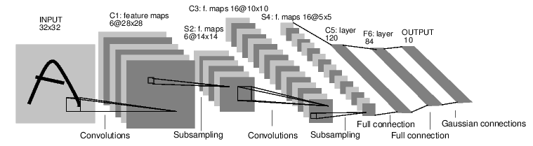
Example: MNIST Convolutional Network
Let's classify some digits!
Define the network
import torch
from torch.autograd import Variable
import torch.nn as nn
import torch.nn.functional as F


class Net(nn.Module):

    def __init__(self):
        super(Net, self).__init__()
        # 1 input image channel, 6 output channels, 5x5 square convolution
        # kernel
        self.conv1 = nn.Conv2d(1, 6, 5)  # 1 input channel = greyscale
        self.conv2 = nn.Conv2d(6, 16, 5)
        # an affine operation: y = Wx + b
        self.fc1 = nn.Linear(16 * 5 * 5, 120)
        self.fc2 = nn.Linear(120, 84)
        self.fc3 = nn.Linear(84, 10)

    def forward(self, x):
        # Max pooling over a (2, 2) window
        x = F.max_pool2d(F.relu(self.conv1(x)), (2, 2))
        # If the size is a square you can only specify a single number
        x = F.max_pool2d(F.relu(self.conv2(x)), 2)
        # reshaping, in this case flatten it
        x = x.view(-1, self.num_flat_features(x))

        # Affine operations
        x = F.relu(self.fc1(x))
        x = F.relu(self.fc2(x))
        x = self.fc3(x)
        return x

    def num_flat_features(self, x):
        size = x.size()[1:]  # all dimensions except the batch dimension
        num_features = 1
        for s in size:
            num_features *= s
        return num_features

net = Net()
net
That is… awesome.
params = list(net.parameters())
params[2].size()
input = Variable(torch.randn(1, 1, 32, 32))  # 32 because ?
out = net(input)
out
net.zero_grad()
out.backward(torch.randn(1, 10))  # initialize weights randomly
=torch.nn only supports mini-matches, not single sample.
For example, nn.Conv2d will take in a 4D Tensor of n_samples x n_channels x height x width.
If you have a single sample, just use input.unsqueeze(0) to add a fake batch dimension.
Loss function
output = net(input)
target = Variable(torch.range(1, 10))  # dummy target
criterion = nn.MSELoss()  # mean-squared-error

loss = criterion(output, target)
loss
Now, if you follow loss in the backward direction, using it’s .creator attribute,
you will see a graph of computations that looks like this:
input -> conv2d -> relu -n> maxpool2d -> conv2d -> relu -> maxpool2d -> view -> linear -> relu -> linear -> relu -> linear -> MSELoss -> loss
So, when we call loss.backward(), the whole graph is differentiated w.r.t. the loss,
and all Variables in the graph will have their .grad Variable accumulated with the gradient.
loss.creator.previous_functions[0][0]
Backprop
net.zero_grad()  # zeros gradient buffers of all parameters
net.conv1.bias.grad
loss.backward()
net.conv1.bias.grad
Again, awesome!
Updating the weights
For simplicity, we'll simply do the standard Stochastic Gradient Descent (SDG).
learning_rate = 0.01
for f in net.parameters():
    f.data.sub_(f.grad.data * learning_rate)
params[0][0][0] # first filter or feature-map of conv1
However, we'll probably like to use different update rules. We can find these in the optim package.
import torch.optim as optim

optimizer = optim.SGD(net.parameters(), lr=0.01)

optimizer.zero_grad()  # zero the gradient buffers
output = net(input)
loss = criterion(output, target)
loss.backward()
optimizer.step()  # does the update
params[0][0][0]
Example: Linear regression
import numpy as np
import matplotlib.pyplot as plt

from sklearn.datasets import make_regression
from sklearn.model_selection import train_test_split
from sklearn.metrics import log_loss

import torch
import torch.nn as nn
from torch.autograd import Variable


RANDOM_SEED = 42
np.random.seed(RANDOM_SEED)


# Hyperparameters
input_size = 1
output_size = 1
epochs_n = 60
alpha = 0.001


# Dataset
X, y = make_regression(n_features=1, random_state=RANDOM_SEED)
X, y = X.astype(np.float32), y.astype(np.float32)
X_train, X_test, y_train, y_test = train_test_split(
    X, y, random_state=RANDOM_SEED)

# Linear regression model
class LinearRegression(nn.Module):
    def __init__(self, input_size, output_size):
        super(LinearRegression, self).__init__()
        self.linear = nn.Linear(input_size, output_size)

    def forward(self, x):
        out = self.linear(x)
        return out


reg_model = LinearRegression(input_size, output_size)

# Training the model
for epoch in range(epochs_n):
    # Convert numpy array to `Variable`
    inputs = Variable(torch.from_numpy(X_train))
    outputs = Variable(torch.from_numpy(y_train))

    # Forward
    predictions = reg_model.forward(inputs)

    # Backward
    reg_model.zero_grad()
    loss = (predictions - outputs).pow(2).sum()
    loss.backward()

    # Update
    reg_model.linear.weight.data -= alpha * reg_model.linear.weight.grad.data
    reg_model.linear.bias.data -= alpha * reg_model.linear.bias.grad.data

predictions_test = reg_model.forward(Variable(torch.from_numpy(X_test))).data.numpy()
print(np.square((y_test - predictions_test)).sum())
print(predictions_test.shape)

plt.plot(X_test, predictions_test, label="pred")
plt.scatter(X_test, y_test, label="true", color="g")
plt.legend()
plt.show()
Example: Feed Forward Neural Network on linear regression
import numpy as np
import matplotlib.pyplot as plt

from sklearn.datasets import make_regression
from sklearn.model_selection import train_test_split
from sklearn.metrics import log_loss

import torch
import torch.nn as nn
import torch.nn.functional as F
from torch.autograd import Variable


RANDOM_SEED = 42
np.random.seed(RANDOM_SEED)


# Hyperparameters
input_size = 1
output_size = 1
epochs_n = 100
batch_size = 20
alpha = 0.001


# Dataset
X, y = make_regression(n_features=input_size, random_state=RANDOM_SEED)
X, y = X.astype(np.float32), y.astype(np.float32)
X_train, X_test, y_train, y_test = train_test_split(
    X, y, random_state=RANDOM_SEED)


class FeedForwardNeuralNetwork(nn.Module):
    def __init__(self, input_size, layer_sizes):
        self.layers = [nn.Linear(input_size, layer_sizes[0])]
        for i in range(len(layer_sizes) - 1):
            l = nn.Linear(*layer_sizes[i:i+2])
            self.layers.append(l)

    def forward(self, x):
        for l in self.layers[:-1]:
            x = F.sigmoid(l(x))

        x = self.layers[-1](x)
        return x

    def zero_grad(self):
        for l in self.layers:
            l.zero_grad()


model = FeedForwardNeuralNetwork(input_size, [20, 30, 1])

# Training the model
for epoch in range(epochs_n):
    # Convert numpy array to `Variable`
    indices = np.random.randint(X_train.shape[0], size=batch_size)
    inputs = Variable(torch.from_numpy(X_train[indices]))
    outputs = Variable(torch.from_numpy(y_train[indices]))

    # Forward
    predictions = model.forward(inputs)

    # Backward
    loss = (predictions - outputs).pow(2).sum()
    loss.backward()

    # Update
    for l in model.layers:
        l.weight.data -= alpha * l.weight.grad.data
        l.bias.data -= alpha * l.bias.grad.data

    model.zero_grad()


predictions_test = model.forward(Variable(torch.from_numpy(X_test))).data.numpy()
print(np.square((y_test - predictions_test)).sum())
print(predictions_test.shape)

plt.scatter(X_test, predictions_test, label="pred")
plt.scatter(X_test, y_test, label="true", color="g")
plt.legend()
plt.show()
Example: Recurrent Neural Network on linear regression
import numpy as np
import matplotlib.pyplot as plt

from sklearn.datasets import make_regression
from sklearn.model_selection import train_test_split
from sklearn.metrics import log_loss

import torch
import torch.nn as nn
import torch.nn.functional as F
from torch.autograd import Variable

from progress.bar import Bar


RANDOM_SEED = 42
np.random.seed(RANDOM_SEED)


# Hyperparameters
input_size = 1
output_size = 1
window_size = 5
hidden_size = 24
# In this particular problem, increasing epochs_n might give you `nan`
# predictions I believe this is due to the extrapolating nature of the problem,
# where we are looking ahead when trying to make predictions on the test data.
epochs_n = 100
alpha = 0.001


# Dataset
X, y = make_regression(n_features=1, random_state=RANDOM_SEED)
X, y = X.astype(np.float32), y.astype(np.float32)
X_train, X_test, y_train, y_test = train_test_split(
    X, y, random_state=RANDOM_SEED
)


class RNN(nn.Module):
    def __init__(self, input_size, output_size, hidden_size):
        super(RNN, self).__init__()

        self.W_hx = nn.Linear(input_size, hidden_size)
        self.W_hh = nn.Linear(hidden_size, hidden_size)
        self.W_hy = nn.Linear(hidden_size, output_size)

        # hidden state
        self.h = Variable(torch.randn(1, hidden_size), requires_grad=True)

    def forward(self, X):
        """`X` is a sequence of observations"""
        for x in X:
            self.h = self.W_hh(self.h) + self.W_hx(x.resize(x.size()[0], 1))
            self.h = F.tanh(self.h)

        return self.W_hy(self.h)


model = RNN(input_size, output_size, hidden_size)

X_train = torch.from_numpy(X_train)
y_train = torch.from_numpy(y_train)
X_test = torch.from_numpy(X_test)
y_test = torch.from_numpy(y_test)


def plot_rnn_predictions(model, X, y=None, window_size=3, **plot_kwargs):
    xs = []
    preds = []

    if y is not None:
        ys = []

    for i in range(1, X_test.size()[0] + 1):
        end_idx = i
        start_idx = max(end_idx - window_size, 0)
        input_seq = Variable(X_test[start_idx: end_idx])
        pred = model.forward(input_seq)
        xs.append(X_test[end_idx - 1][0])
        preds.append(pred.data.squeeze()[0])

        if y is not None:
            ys.append(y[end_idx - 1])

    plt.scatter(xs, preds, **plot_kwargs)

    if y is not None:
        plt.scatter(xs, ys, label="true", color="g")


plot_rnn_predictions(model, X_test, window_size=window_size,
                     label="pre-train", color="r")

losses = []
bar = Bar("Epoch", max=epochs_n)
for epoch in range(epochs_n):
    # progress
    bar.next()

    # on second thought: we would probably get better performance,
    # or rather faster convergence, if we trained on entire dataset
    # and predict some output after each step. This would allows us
    # to fit the hidden layer `h` on EACH STEP, rather than after
    # each `window_size` sequence-step.
    # ACTUALLY this might pose an issue when using PyTorch, as the
    # autograd would backpropagate aaaaall the way back.
    # Thus, we ought to do exactly what we do now, but of course
    # run through all of the time-steps.
    end_idx = np.random.randint(1, X_train.size()[0] + 1)
    start_idx = max(end_idx - window_size, 0)
    inputs = Variable(X_train[start_idx: end_idx])
    output = y_train[end_idx - 1]

    # Forward
    pred = model.forward(inputs)

    # Backward
    loss = (pred - output).pow(2)
    losses.append(loss.data.squeeze()[0])
    loss.backward(retain_variables=True)

    # Update
    model.W_hx.weight.data -= alpha * model.W_hx.weight.grad.data
    model.W_hx.bias.data -= alpha * model.W_hx.bias.grad.data

    model.W_hh.weight.data -= alpha * model.W_hh.weight.grad.data
    model.W_hh.bias.data -= alpha * model.W_hh.bias.grad.data

    model.W_hy.weight.data -= alpha * model.W_hy.weight.grad.data
    model.W_hy.bias.data -= alpha * model.W_hy.bias.grad.data

    model.h.data -= alpha * model.h.grad.data

    model.zero_grad()


plot_rnn_predictions(model, X_test, y=y_test, window_size=window_size,
                     label="predictions", color="b")
plt.suptitle("Recurrent Neural Network")
plt.title("Linear regression with window size of %d" % window_size)
plt.legend()
plt.show()

# setting the title for some reason messed up the previous plot
# and I'm not bothered to fix this right now :)
# Hence => don't add title!
plt.scatter(range(len(losses)), losses)
plt.title("Losses over %d epochs" % epochs_n)
plt.xlabel("epoch")
plt.ylabel("loss")
plt.show()

# progress.bar does not add a newline to the end, so we fix
print()
Appendix A: Definitions
- Affine operation
- operation on the affine space, which is a generalization of the Euclidean space that are independent of the concepts of distance and measure of angles, keeping only the properties related to parallelism and ratio of lengths for parallel line segments. Note: Euclidean space is an affine space.