Optimization
Table of Contents
Notation
 - learning rate
 - cost of using
  to approximate the real function
  for observed input-output pairs
  and
and 
 - approx. value for
  after
after  iterations
First-order
Overview
First-order optimization techniques only take into account the the first-order derivative (the Jacobian).
These kind of methods are of course usually slower than the second-order techniques, but posess the advantage of being much more feasible for high-dimensional data.
Consider some  weight matrix
  . Taking the derivative
of some function
. Taking the derivative
of some function  gives us a
Jacobian matrix of dimensions, i.e.
gives us a
Jacobian matrix of dimensions, i.e.  derivatives.
If we want the Hessian, we then have to take the partial derivatives
of all the combinations of the Jacobian, givig us a total of
derivatives.
If we want the Hessian, we then have to take the partial derivatives
of all the combinations of the Jacobian, givig us a total of  partial derivatives to compute. See the issue?
Gradient Descent
Motivation
- Finding minimum of some arbitrary function without having to compute the second-order derivative
- Preferable iterative method, allowing incremental improvements
Definition
 1
1
where
 is some arbitrary function
- is the learning-rate
Typically in machine learning we want to minimize the cost of some function  over some parameters , which we might denote
  (in my opinion, more precisely
  ).
Usually we don't have access to the entire function but samples of input-output pairs.
Therefore we cannot compute the full gradient of and need to somehow approximate
the gradient. And so Batch Gradient Descent arises!
).
Usually we don't have access to the entire function but samples of input-output pairs.
Therefore we cannot compute the full gradient of and need to somehow approximate
the gradient. And so Batch Gradient Descent arises!
Batch Gradient Descent
Motivation
- Perform gradient descent without having to know the entire function we're approximating
Definition
 2
2
where the gradient now is the average over all observations 
Issues
- Expensive to compute average gradient across entire set of observations
- Convergence tends to be slow as some data where our prediction is way off might be "hidden" away in the average
Stochastic Gradient Descent
Motivation
- Computing the full approximation to the gradient in Batch Gradient Descent is expensive
- Also want to address the issue of potentially "hidden" away mistakes we're making
Definition
 3
3
where now the gradient is compute from a single observation.
Issues
- Usually quite unstable due to high variance
- Can be mitigated by decreasing the learning rate as we go, but this has the disadvantage of vanishing gradient
Mini-batch Gradient Descent
These days, when people refer to Stochastic Gradient Descent (SGD) they most of the time mean Mini-batch Gradient Descent. It's just generally much better.
Motivation
- Reduce instability (variance) of Stochastic Gradient Descent
- Improve the slow & expensive Batch Gradient Descent
- Make use of highly optimized matrix-operations
Definition
 4
4
where  is the size of the mini-batch.
Issues
- Choosing proper learning-rate is hard
- SGD only guarantees convergence local minimas for non-convex functions,
and can easily be "trapped" in these local minimas
- In fact, saddle-points are argued to be a larger problem, as the gradient is zero in all dimensions, making it hard for SGD to "escape" / "get over the edge and keep rolling"
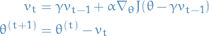
Momentum SGD
Motivation
- If we keep seeing that is a "good thing" to update in some direction, then it would make sense to perform larger updates in this direction
Definition
 5
5
I really suggest having a look at Why Momentum Really Works by Gabriel Goh. It provides some theoretical background to why this simple addition works so well, in combinations with a bunch of visualizations to play with.
Issues
- We have tendency to "overshoot" since we now have this "velocity" component, leading to oscillations around the point of convergence instead of reaching it and staying there. This is especially an issue for non-convex functions as we might actually overshoot the global minima.
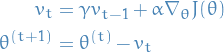
Nestorov Momentum SGD
Motivation
- Better control the overshooting of Momentum SGD
Definition
 6
6
Here we approximate the next value of ( ) by evaluating
the gradient at the current point,
) by evaluating
the gradient at the current point,  , minus the momentum-term we'll
be adding,
, minus the momentum-term we'll
be adding,  , to obtain . In this way we get a certain control
of the step we're taking by "looking ahead" and re-adjusting our update.
, to obtain . In this way we get a certain control
of the step we're taking by "looking ahead" and re-adjusting our update.
If the update  is indeed a "bad" update, then
  will point towards again, correcting some of the "bad" update.
Sometimes people swaps the + sign in the update, like in the paper I'm about to suggest that you have a look at:
Have a look at Ilya Sutskever's thesis in section 7.2 where you get a more mathematical description of why this is a good idea.
Adagrad
Motivation
- We would like to adapt our updates to each individual parameter to perform larger
or smaller updates depending on the importance of the parameter
- Say you barely see this one parameter in your updates, but then suddenly you look at an observation where this parameter has a significant impact. In this case it would make sense to perform a greater-than-normal update for this parameter.
- We still don't like the fact that all previous methods makes us have to manually
tune the learning rate
Definition
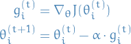 7
7
where  denotes the ith component of .
Or better:
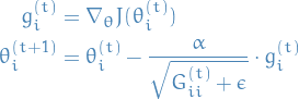 8
8
where
 is a diagonal matrix where each diagonal element
  is the
sum of the squares of the gradients w.r.t. up to
is the
sum of the squares of the gradients w.r.t. up to  is a smoothing term that avoids zero-division (usually on the order of
  )
)
Finally to make use of efficient matrix-operations:
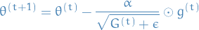 9
9
Issues
- Accumulation of the squared gradient in the denominator means that eventually the denominator will so large that the learning-rate goes to zero
RMSProp
Motivation
- Fix the issue of the too aggressive and monotonically decreasing learning rate of Adagrad
Definition
Issues
Adam (usually the best)
Second-order
Resources
- An overview of gradient descent optimization algorithms A great blog-post providing an overview as the title says.
- Why Momentum Really Works A fantastic post about momentum in SGD. Provides some nice theoretical footing for its efficiency and really cool visualizations.