Nonparametric Bayes
Table of Contents
Concepts
- Infinitively exchangeable
- order of data does not matter for the joint distribution.
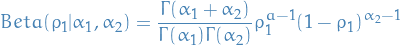
Beta distribution
 1
1
Overview
- Distribution over parameters for a binomial-distribution!
- So in a sense you're "drawing distributions"
- Like to think of it as simply putting some rv. parameters on the model
itself, instead of simply going straight for estimating
 in a binomial
distribution.
in a binomial
distribution.
- Remember the
 function is a
 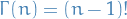 when
when  is an integer.
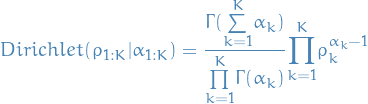
Dirichlet distribution
 2
2
Overview
- Generialization of Beta distribution, i.e. over multiple categorical variables, i.e. distribution over parameters for a multionomial distribution.
- So if you say were to plot the Dirichlet distribution of some parameters
 we obtain the simplex/surface of allowed values for these parameters
- "Allowed" meaning that they satisfy being a probability within the multinomial
model, i.e.
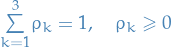
- "Allowed" meaning that they satisfy being a probability within the multinomial
model, i.e.
- Got nice conjugacy properties, where it's conjugate to itself, and also multinomial distributions
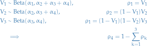
Generating Dirichlet from Beta
We can draw from a Beta by marginalizing over 
 3
3
This is what we call stick braking.
 4
4
Dirichlet process
Overview
- Taking the number of parameters
 to go to
  .
. - Allows arbitrary number of clusters => can grow with the data
Taking 
We do what we do in Generating Dirichlet from Beta, the "stick braking". But in the Dirichlet process stick braking we do
 5
5
And then we just continue doing this, drawing  as follows:
![\begin{equation*}
V_k \sim \text{Beta}(a_k, b_k), \qquad
\rho_k = \Bigg[ \overset{k - 1}{\underset{j=1}{\prod}} (1 - V_j) \Bigg] V_k
\end{equation*}](../../assets/latex/nonparameteric_bayes_5c39a18f6158e36f12245f0b87c518bfe7c87e4a.png) 6
6
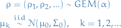
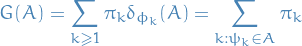
Resulting distribution of is then
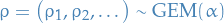
where  is called the Griffiths-Engen-McCloskey (GEM) distribution.
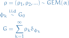
To obtain a Dirichlet process we then do:
 7
7
where  can be any probability measure.
Dirichlet process mixture model
Start out with Gaussian Mixture Model
 8
8
Where our  and
and  are our priors of the Gaussian clusters.
Which is the same as saying
are our priors of the Gaussian clusters.
Which is the same as saying 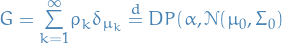 .
.
So, is a sum over dirac deltas and so will only take non-zero
values where  corresponds to some . That is, it just
indexes the probabilities somehow. Or rather, it describes the
probability of each cluster being assigned to.
corresponds to some . That is, it just
indexes the probabilities somehow. Or rather, it describes the
probability of each cluster being assigned to.
 9
9
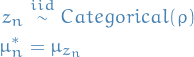
i.e.  , which means that drawing an assignment cluster for our
nth data point, where the drawn cluster has mean
, which means that drawing an assignment cluster for our
nth data point, where the drawn cluster has mean  , is equivalent of drawing
the mean itself from .
, is equivalent of drawing
the mean itself from .
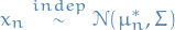
i.e. the nth data point is then drawn from a normal distribution with
the sampled mean  and some variance
  .
.
The shape / variance could also be dependent on the cluster if we wanted
to make the model a bit more complex. Would just have to add some draw for
in our model.
Lecture 2
Notation
 which sums to 1 with probability one.
 is the dirac delta for the element
Stuff
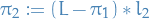
- can be described as follows:
- Take a stick of length


- "Break" stick at the point corresponding to
 :
:
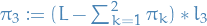
- "Break" the rest of the stick by
 :
:
- "Break" the rest of the stick:
- …
Then

- Take a stick of length
We let

where
 is some underlying distribution
The we define the random variable
where
is the dirac delta for the element
- The can even be functions, if is a distribution on a separable Banach space!
- The
Then

where
 denotes a Dirichlet process
Observe that
defines a measure!
hence a
is basically a distribution over measures!
So we have a random measure where the σ-algebra is defined by
where
 is the original σ-algebra

There's a very interesting property of the distribution.
Suppose  is Brownian motion. Then consider the maximal points (i.e. new "highest" or "lowest" peak), then the time between these new peaks follow a !
We say a that a sequence of random variables  is infinitely exchangable if and only if there exists an unique random measure such that
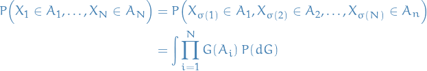
Then observe that what's known as the Chinese restaurant process is just our previous 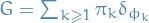 where we've marginalized over all the
  !
!
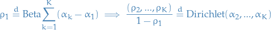
Dirichlet as a GEM
Suppose we have finite number of samples from a GEM distribution  .
.
Then,

Stochastic process on a σ-algebra.
A complete random measure is a random measure such that the draws are independent:
Appendix A: Vocabulary
- categorical distribution
- distribution with some probability for the
the class/label indexed by . So a multinomial distribution?
- random measure