Neural Networks
Table of Contents
Neural Networks
If you ever want to deduce the backpropagation-algorithm yourself, DO NOT ATTEMPT TO DO IT USING MATRIX- AND VECTOR-NOTATION!!!!
It makes it sooo much harder. If you check out the Summary you can see the equations in matrix- and vector-form, but these were deduced elementwise and then transformed into this notation due to the efficient nature of these operations rather than elementwise operations.
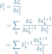
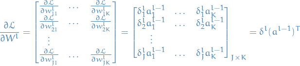
Backpropagation
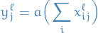
Notation
 is our prediction / final output
 is what it's supposed to be, i.e. the real
output
is what it's supposed to be, i.e. the real
output the output of the
  layer
layer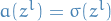 , in this case, not necessary in general
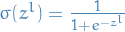
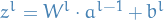
 weight matrix between the
  and
layer
and
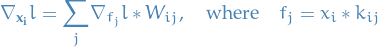
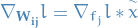
layer is the
  row of s.t.
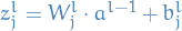
Method
This my friends, is backpropagation.
We have some loss-function  , which we set to be the
least-squares loss just to be concrete:
, which we set to be the
least-squares loss just to be concrete:
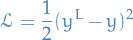 1
1
We're interested in how our loss-function for some prediction changes wrt. to the weights in all the different layers, right?
We start at the back, with the error of the last layer  :
:
 2
2
We then let 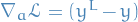 (dropping the subscript, as we now
consider a vector of outputs), and write
(dropping the subscript, as we now
consider a vector of outputs), and write
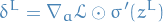 3
3
Where the Hadamar-product is simply a element-wise product.
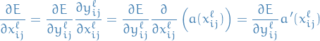
Next, we need to obtain an expression for the error in the
 layer as a function of the next layer,
i.e. the
layer as a function of the next layer,
i.e. the  layer.
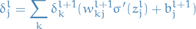
Consider the error  for the
  activation
/ neuron in the layer.
activation
/ neuron in the layer.
 4
4
With this recursive relationship we can start from the back,
since we already know  , and work our way to the
actual input to the entire network.
, and work our way to the
actual input to the entire network.
Still got to obtain an expression for  !
!
 is simply given by all the
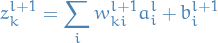 5
5
Taking the derivative of this wrt. 
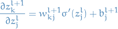 6
6
due to 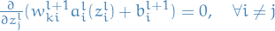 .
.
Substituting back into the expression for
 7
7
And finally rewriting in matrix-form:
 8
8
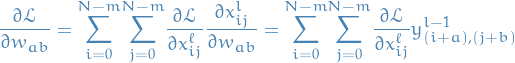
So, we now have the following expressions:
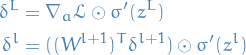 9
9
We have our recursive relationship between the errors in the layers, and the error in the final layer, allowing us to compute the errors in the preceding layers using the recursion.
But the entire reason for why all this is interesting is
that we want to obtain an expression for how to update
the weights and biases  in each layer to improve
(i.e. reduce) these errors!
in each layer to improve
(i.e. reduce) these errors!
That is; we want some expressions for  and
and  .
.
 10
10
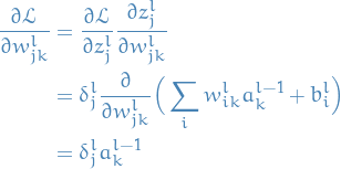
Let's turn this into vector-notation for each row in .
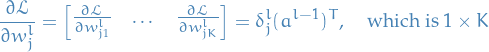 11
11
And finally a full-blown matrix-notation:
 12
12
And from the second-to-last line in the previous equation
we see that if we instead take the partial-derivative wrt.
 we obtain
 13
13
Summary
And we end up with the following equations, using matrix notation:
 14
14
Convolutional Neural Networks (CNN)
Have the following properties:
Local connectivity
Each hidden unit look at small part of image, i.e. we have small window / "receptive field" which each hidden unit ("neuron") looks at. In image-recognition, each neuron looks at a different "square" of the image.
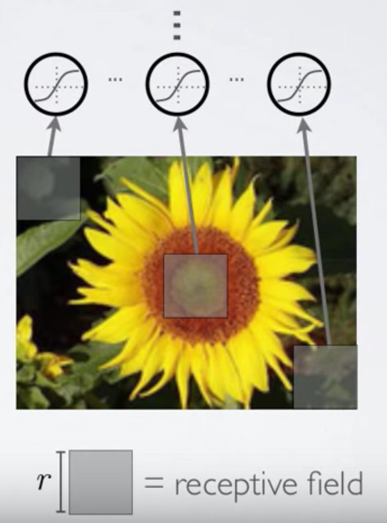
This means that each hidden unit will have one weight / connection for each pixel or data-point in the receptive field.
In the case where each pixel or data-point is of multiple dimensions,
we will have a connection from each of these dimension, i.e. for N
dimensional data-points we have N * (area of receptive field) weights / connections.
Why
- Fully connected hidden layer would have an unmanageable number of parameters
- Computing the linear activations of the hidden units would be computational very expensive
Parameter sharing
Share matrix of parameters / weights across certain hidden units. That is; we define a feature map which is a set of hidden units that share parameters. All hidden units in the same feature map are looking at separate parts of the image. Typically the hidden units in a feature map together covers the entire image. This is also referred to as a filter I believe.
Notation
- channel is the "data-point" which can be of multiple dimensions. Used because of the typical input for an image being RGB-channels.
 input channel, specifies which dimension of the input / "data-point"
we're considering
input channel, specifies which dimension of the input / "data-point"
we're considering- feature map
 is the input channel
 is the matrix connecting the input channel
to the feature map, i.e. with RGB-channels
is the matrix connecting the input channel
to the feature map, i.e. with RGB-channels  corresponds to the red-channel (
 ) and 2nd feature map (
 )
) is the convolution kernel (matrix)
 means
means  with rows and columns flipped
 is the learning factor
 is the hidden layer
 convolution operation
 convolution operation with zero-padding
 is a (usually non-linear) activation function,
e.g.
is a (usually non-linear) activation function,
e.g. sigmoid,ReLUandtanh.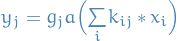 , is not always used
Why
- Reduces the number of parameters further
- Each feature map or filter will extract the same feature at each different position in the image. Feature are equivariant.
Discrete convolution
Why do we use it in a Convolution Network?
We have a connection between each input (channel) and hidden unit in a feature map. We want to compute the element-wise multiplication between the input matrix and the weight-matrix, then sum all the entries in the resulting matrix.
If we flip the rows and columns of the weight-matrix, this operation corresponds to taking the convolution operation between this flipped matrix and the inputs.
Why do we want to do that? Efficiency. The convolution operation is something which is heavily used in signal processing, and so we can easily take advantage of previous techniques for computing this product.
This is really why we use the convolution operation, and why it's called, well, a convolutional network.
Pooling / subsampling hidden units
- Performed in non-overlapping neighborhoods (subsampling)
- Aggregate results from this neighborhood
Maximum pooling
Take the maximum value found in this neighborhood
Average pooling
Compute the average of the neighborhood.
Subsampling
- Generalization of average pooling
- Average pooling with learnable weights for each filter map
Back-propagation
For some loss-function  we can use back-propogation to compute
the total loss for a prediction.
we can use back-propogation to compute
the total loss for a prediction.
Here we are only working on a single input at the time.
Generalizing to multiple inputs would simply be to also sum over
all  , yeah?
For a convolutional layer we have the following:
 15
15
describes the change in the loss wrt. the input channel, and
 16
16
Clearer deduction
Instead one might consider the explicit sums instead of looking at the convolution operation.
Consider the equations for forward propagation:
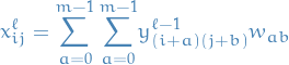 17
17
where:
 is the pre-activations or pre-non-linearities used by the
  layer,
which is a convolutional layer.
layer,
which is a convolutional layer. is an entry in the weight-matrix for the correspondig feature-map or filter
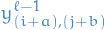 is the activation or non-linearity from the previous layer,
which can be any type of layer (pooling, convolutional, etc.)
is the activation or non-linearity from the previous layer,
which can be any type of layer (pooling, convolutional, etc.)
Then the activation of the feature-map / filter in the layer
(a convolutional layer) is:
 18
18
Could also have some learning rate multiplied by .
Now, for backward propagation we have:
 19
19
for each entry in the weight matrix for each feature-map.
Note the following:
- This double sum corresponds to accumulating the loss for the weight
- Sum over all expressions in which occurs (corresponds to weight-sharing)
And since the above expression depends on we need to compute that!
 20
20
There you go! And we already know the error on the layer, so we're good!
And when doing back-propagation we need to describe the loss for some layer
wrt. to the next layer,  :
:
 21
21
where we note that:
- came from the definition for the forward-propagation
- expression looks slightly like it could be expressed using convolution, but instead
of having
 we have
  .
. - expression only makes sense for points that are at least
 away from the top
and left edges (because
away from the top
and left edges (because  and
and  mate)
mate)
We solve these problems by:
- pad the top and left edges with zeros
- then flip axes of

and then we can express this using the convolution operation! (which I'm not showing, because I couldn't figure out how to it. I was tired, mkay?!)
Q & A
DONE Why is the factor of in the derivative of the loss-function wrt. for a convolutional layer not with axes swapped?
Have a look at the derivation here. (based on this blog post) Basically, it's easier to see what's going on if you consider the actual sums, instead of looking at the kernel operation, in my opinion.
DONE View on filters / feature-maps and weight- or parameter-sharing
First we ignore the entire concept of feature-maps / filters.
You can view the weight- or parameter-sharing in two ways:
- We have one neuron / hidden unit for each window, i.e. everytime you move the window
you are using a new neuron / hidden unit to view pixels / data-points inside the window.
Then you think about all of this aaand:
- There is in fact nothing special with a neuron / hidden unit, but rather the weights it uses for it's computation (assuming these neurons have the same activation function).
- If we then are to make all these different neurons use the same weights, voilá! We have our weight-sharing!
- We have one neuron / hidden unit with its weight-matrix for its receptive field / window. As we slide over, we simply move the neuron and it's connections with us.
In the 1st "view", the feature-map / filter corresponds to all these separate neurons / hidden-units which use the same weight-matrix, and having multiple feature-maps / filters corresponds to having multiple such sets of neurons / hidden units with their corresponding weight-matrix.
In the 2nd "view", the feature-map / filter is just a specific weight-matrix, and having multiple independent weight-matrices corresponds to having multiple feature-maps / filters.
Generative Adversarial Networks (GAN)
Notation
 - generative model that captures the data distribution, a mapping to the input space
 - discriminative model that estimates the probability that a sample
came from the data rather than
- discriminative model that estimates the probability that a sample
came from the data rather than  - single value representing the probability that
  came from the data (i.e. is "real") rather than generated by
  - parameter for
  - parameter for
  - distribution estimated by the generator
  or
or  - distribution over the real data
 - distribution from where we sample inputs to the generative model , i.e. the output-sample from is
  , i.e. the distribution over the noise used by the generator
Overview
- Goal is to train to be so good at generating samples that really can't tell
whether or not the input came from or is "real"
- Example: inputs are pictures of dogs → learns to generate pictures of dogs
so well that can't tell if it's actually a "real" picture of a dog or one generated
by
- Example: inputs are pictures of dogs →
- In the space of arbitrary functions and , a unique solution exists,
with recovering the training data distribution (
 )
)
Cost
Kullback-Leibner Divergence
In other words, and play the following two-player minimax game with
value function  :
:
![\begin{equation*}
\min_G \max_D V(D, G) =
\mathbb{E}_{\mathbf{x} \sim p_{\text{data}} (\mathbf{x})} [\log D(\mathbf{x})] +
\mathbb{E}_{\mathbf{z} \sim p_{\mathbf{z}}(\mathbf{z})} [\log (1 - D(G(\mathbf{z})))]
\end{equation*}](../../assets/latex/neural_networks_6d04f1ea57d1cfbe99ef7d2927cad6ac10be0256.png) 22
22
Remember that this actually is optimizing over and ,
the parameters of the models.
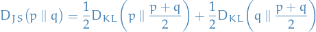
Jensen-Shannon Divergence
I wasn't aware of this when I first wrote the notes on GANs, hence there might be some changes which needs to be made in the rest of the document to accomodate (especially to the algorithm section, as this uses the derivative of KL-divergence).
There is a "problem" with the KL-divergence; it's asymmetric. That is, if  is close to zero, but
  is signficantly non-zero, the effect of
  is disregarded.
Jensen-Shannon divergence is another measure of similiarity between two distributions, which have the following properties:
- bounded by $[0, 1]
- symmetric
- smooth(er than KL-divergence)
Training
- and are playing a minimax game
- Optimizing in completion in the inner loop of training is computationally
prohibitive and on finite datasets would lead to overfitting
- Solution: alternate between
 steps of optimizing and one
step optimizing
steps of optimizing and one
step optimizing
- is maintained near its optimal solution, as long as converges slowly enough
Optimal value for , the discriminator
The loss function is given by

We're currently interested in maximizing  wrt.
wrt.  , thus

where we've assumed it's alright to interchange the integration and derivative. This gives us
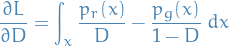
Setting equal to zero, we get
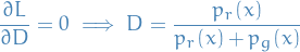
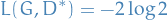
If we then assume that the generator is trained to optimality, then  , thus

is the optimal value wrt. alone.
In this case, we the loss is given by
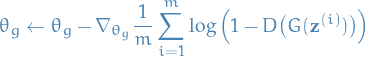
Algorithm
Minibatch SGD training of GANs. The number of steps to apply to the discriminator
in the inner loop, , is a hyperparameter. Least expensive option is  .
.
for number of training iterations do
- for steps do
- Sample minibatch of noise samples
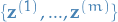 from noise prior
- Sample minibatch of examples
 from data distribution
Update
by ascending its stochastic gradient:
![\begin{equation*}
\theta_d \leftarrow \theta_d + \nabla_{\theta_d} \frac{1}{m} \sum_{i=1}^m \Big[ \log D(\mathbf{x}^{(i)}) + \log \Big( 1 - D \big( G(\mathbf{z}^{(i)}) \big) \Big) \Big]
\end{equation*}](../../assets/latex/neural_networks_7598d490c9511488435dd7ff37c30c4b4a8f0135.png) 23
23
- Sample minibatch of
- end for
- Sample minibatch of noise samples from noise prior
Update the generator by descending its stochastic gradient:
 24
24
end for
This demonstrates a standard SGD, but we can replace the update steps with any stochastic gradient-based optimization methods (SGD with momentum, etc.).
Implementation
Issues
Nash equilibrium: hard to achieve
- Updating procedure is normally executed by updating both models using their respective gradients jointly
- If and are updated in completely opposite directions, there's a real danger of getting oscillating behavior, and if you're unlucky, this might even diverge
Low dimensional supports
- Dimensions of many real-world datasets, as represented by , only appear to be artificially high
- Most datasets concentrate in a lower-dimensional manifold
- also lies in low dimensional manifold due to (usually) the random nuber used by is low-dimensional
- both and are low-dimensional manifolds => almost certainly disjoint
- In fact, when they have disjoint support (set not mapped to zero), we're always capable of finding perfect discriminator that separates real and fake samples 100% correctly
Vanishing gradient
- If discriminator is perfect =>
 goes to zero => no gradient loss
Thus, we have dilemma:
- If behaves badly, generator doesn not have accurate feedback and the loss function cannot represent reality
- If does a great job, gradient of the loss function drops too rapidly, slowing down training
Mode collapse
- may collapse to a setting where it always produces same outputs
Improving GAN training
Wasserstein GAN (WGAN)
Attention
Activation functions
Notation
 is the pre-activation, with
  being the jth component
Sigmoid
Definition
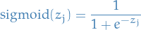 25
25
Rectified Linear Unit (ReLu)
Definition
 26
26
Pros & cons
- No vanishing gradient
- But we might have exploding gradients
- Sparsity
Notes
- Exploding gradients can be mitigated by "clipping" the gradients, i.e. setting an upper- and lower-limit for the value of the gradient
- There are multiple variants of ReLU, where most of them include a small non-zero gradient when the unit is not active
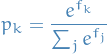
Softmax
Definition
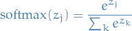 27
27
Pros & cons
- Provides a normalized probability-distribution over the activations
- When viewed in a cross-entropy cost-model, the gradients for the loss-function is cheap computationally and numerical stable
Notes
- Usually only used in the top (output) layer
Exponential Linear Unit (ELU)
Definition
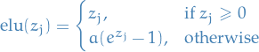 28
28
where  and is a hyper-parameter.
Pros & cons
- Attempts to make the mean activations closer to zero which speeds up learning
- All the pros of ReLU
Notes
- Shown to have improved performance compared to standard ReLU
Scaled Exponential Linear Unit (SELU) [NEW]
Defintion
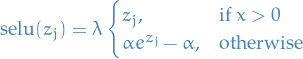 29
29
Pros & cons
- Allows us to construct a Self-normalizing Neural Network (SNN), which attempts to make the mean activations closer to zero and the variance of the activiations close to 1. This is supposed to (and experiments show) greatly increase the stability and efficiency of training.
Notes
- Extension of ELU
- Recent discovery, see Self-Normalizing Neural Networks paper
Loss functions
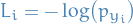
Softmax
Notation
- - ith training sample
 -
-
Definition
- Corresponds to cross-entropy loss
 30
30
Derivtive wrt. cross-entropy loss
Cross-entropy loss function:
 31
31
With  being a softmax:
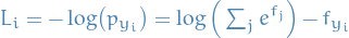
And thus,
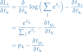 32
32
Thus,
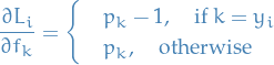 33
33
And a bit more compactly,
 34
34
Resources
- Amazing overview of everything regarding Feed-forward and convolutional networks. Also includes implementation tips, a range of regularization methods and optimization methods.
- CS231 course-notes from Stanford Provides a fantastic overview of everything from activiaton-, loss-functions and different neural network architectures.