Kullback Leibler Divergence
Table of Contents
Definition
Let  and
and  be two probability distributions for a random variable
  .
.
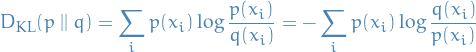
The Kullback-Leibler (KL) divergence
if
is discrete, is given by
if
is continuous,

Interpretation
Probability
Kullback-Leibner divergence from some probability-distributions  and
and  , denoted
  ,
is a measure of the information gained when one revises one's beliefs from the prior distribution
to the posterior distribution . In other words, amount of information lost when
is used to approximate .
,
is a measure of the information gained when one revises one's beliefs from the prior distribution
to the posterior distribution . In other words, amount of information lost when
is used to approximate .
Most importantly, the KL-divergence can be written
![\begin{equation*}
D_{\rm{KL}}(p \ || \ q) = \mathbb{E}_p\Bigg[\log \frac{p(x \mid \theta^*)}{q(x \mid \theta)} \Bigg] = \mathbb{E}_p \big[ \log p(x \mid \theta^*) \big] - \mathbb{E}_p \big[ \log q(x \mid \theta) \big]
\end{equation*}](../../assets/latex/kullback_leibler_divergence_bf4cacc304ab57b5792eb66e803c948e203e94f0.png)
where  is the optimal parameter and
  is the one we vary to approximate
  . The second term in the equation above is the only one which depend on the "unknown" parameter ( is fixed, since this is the parameter we assume to take on). Now, suppose we have
  samples
  from , then observe that the negative log-likelihood for some parametrizable distribution is given by
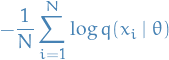
By the Law of Large numbers, we have
![\begin{equation*}
\lim_{N \to \infty} - \frac{1}{N} \sum_{i=1}^{N} \log q(x_i \mid \theta) = - \mathbb{E}_p[\log q(x \mid \theta)]
\end{equation*}](../../assets/latex/kullback_leibler_divergence_96e04ce0e8b58d7c798481548bd91823470368e0.png)
where  denotes the expectation over the probability density . But this is exactly the second term in the KL-divergence! Hence, minimizing the KL-divergence between
  and
and  is equivalent of minimizing the negative log-likeliood, or equivalently, maximizing the likelihood!
Coding
The Kraft-McMillan theorem establishes than any decodable coding scheme for coding a message to identify one value
out of a set of possibilities
over
is the length of the code for
Therefore, we can interpret the Kullback-Leibner divergence as the expected extra message-length per datum that must be commincated if a code that is optimal for a given (wrong) distribution
Let's break this a bit down:
- Kraft-McMillan theorem basically says when taking the exponential of the length of each valid "codeword", the resulting set (of exponentials) looks like a probability mass function.
- If we were to create a coding schema for the values in (our set of symbols) using binary representation (bits) using our "suggested" probability distribution , KL-divergence gives us the expected extra message-length ber datum compared to using a code based on the true distribution