Gaussian Processes for Machine Learning
Table of Contents
Introduction
Gaussian processes is a generalization of Gaussian probability distribution to continuous case where we deal with these infinite number of functions by only considering a finite number of points.
Two common appraoches to deal with supervised learning:
- Restrict the class of functions that we consider
- Prior probability to every possible function
- How do we compare a infinite number of functions?
A Pictorial Introduction to Bayesian Modelling
1D regression
- Here we specify a prior over functions specified by a particular Gaussian process which favours smooth functions
- We assume a 0 mean for every
x, since we don't have any prior knowledge - We then add two data points
 and only consider functions passing through these two points,
ending up with the posterior in 1.1 b
and only consider functions passing through these two points,
ending up with the posterior in 1.1 b
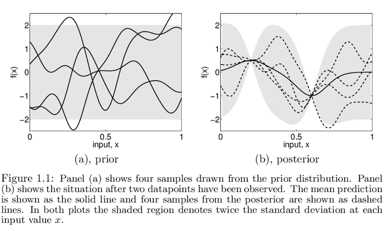
Figure 1: From rasmussen2006gaussian
Regression
There are multiple ways to interpret a Gaussian process (GP)
Weight-space view
Notation
 is
is  of
of  observations
 = input vector of dimension
 = scalar output/target
 =
=  design matrix with all input vectors
as column vectors
design matrix with all input vectors
as column vectors 

Standard Linear Model
Bayesian analysis of the standard linear regression model with Gaussian noise:
 1
1
- Often a bias is included, but this can easily be implemented by adding
a extra element to the input vector , whose value is always

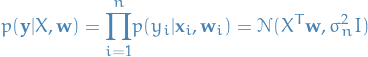
- The noise assumption (
 to be normally distributed) together
with the model direcly gives us the likelihood, ergo the probability
density of the observations given the parameters.
to be normally distributed) together
with the model direcly gives us the likelihood, ergo the probability
density of the observations given the parameters.
Because of (assumed) independence between samples:
 2
2
In the Bayesian formalism we need to specify a prior over the parameters,
expressing our beliefs about the parameters before considering the observations.
We simply give a zero mean Gaussian with covariance matrix  on the weights
 3
3
Inference in a Bayesian linear model is based on the posterior distribution over the weights:
 4
4
where the normalization constant or marginal likelihood is given by
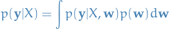 5
5
If we can obtain  without explicitly calculating this integral,
this is what they call "integrating out the weights".
without explicitly calculating this integral,
this is what they call "integrating out the weights".
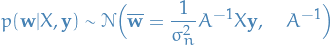
For now we ignore the marginal distribution in the denominator, and then we have
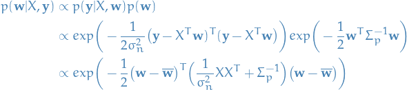 6
6
where  .
Notice how this has the form of a Gaussian posterior with mean
.
Notice how this has the form of a Gaussian posterior with mean  and covariance matrix
  :
:
 7
7
where 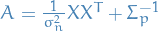 .
.
I suppose this is legit without having to compute the marginal likelihood since we can easily obtain the normalization constant for a Gaussian Distribution.
For this model, and indeed for any Guassian posterior, the mean
of the posterior  is also its mode,
which is also called the maximum a posteriori (MAP) estimate of
is also its mode,
which is also called the maximum a posteriori (MAP) estimate of  .
.
The meaning of the log prior and the MAP estimate substantially differs between Bayesian and non-Bayesian settings:
- Bayesian MAP estimate plays no special role
- Non-Bayesian negative prior is sometimes used as penalty term, and
MAP point is known as the penalized maxium likelihood estimate
of the weights. In fact, this is what is known as ridge regression,
because of the quadratic term
 from the log prior.
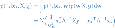
To make predictions for some input  , we average over all the
parameter values, weighted by their posterior probability. Thus the
predictive distribution for
, we average over all the
parameter values, weighted by their posterior probability. Thus the
predictive distribution for  , is given by
averaging (or rather, taking the expectation for
, is given by
averaging (or rather, taking the expectation for  over the
weights
over the
weights  ) the output of all possible linear models w.r.t. the
Gaussian posterior
) the output of all possible linear models w.r.t. the
Gaussian posterior
 8
8
And even the predictive distribution is Gaussian! With a mean given by the posterior mean of the weights from eq. (2.8) multiplied by the new input. All hail Gauss!
The above step demonstrates a crucial part: we can consider all possible weights simply by "integrating out" or "marginalizing over" the weights.
Also note how the predictive variance is a quadratic of the new input, and so the prediction will be more uncertain as the magnitude of test input grows.
Projections of Inputs into Feature Space
- Can overcome linearity by projecting features into higher-dimensional space allowing us to implement polynomial regression
- If projections are independent of parameters => model is still linear in the parameters
and therefore analytically solvable/tractable!
- Data which is not linearly separable in the original data space may become linearly separable in a high dimensional feature space.
Function-space view
Our other approach is to consider inference directly in the function space, i.e. use a GP to describe a distribution over functions.
A Gaussian process is a collection of random variables, any finite number of which have a joint Gaussian distribution.
A GP is completely specified by its mean function  and
covariance function
and
covariance function  . For a real process
![\begin{equation*}
\begin{split}
m(\mathbf{x}) &= E[f(\mathbf{x})] \\
k(\mathbf{x}, \mathbf{x'}) &= E[(f(\mathbf{x}) - m (\mathbf{x}))(f(\mathbf{x'}) - m (\mathbf{x'}))] \\
\end{split}
\end{equation*}](../../assets/latex/gaussian_processes_for_machine_learning_6dbcaf36bb18e84b65c93907c885cb64841618f2.png) 9
9
and we write the Gaussian process as
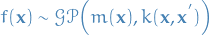 10
10
Usually, for notational simplicity we will take  ,
though this need-not be done.
,
though this need-not be done.
Consistency requirement / marginalization property
GP is defined as collection of rvs a consistency requirement.
This simply means that if the GP e.g. specifies  ,
,

The defintion does not exclude GPs with finite index sets (which would just be Gaussian distributions).
Simple example
Example of GP can be obtained from our Bayesian linear regression model  with prior
  .
.
![\begin{equation*}
\begin{split}
E[f(\mathbf{x})] &= \psi(\mathbf{x})^T E[\mathbf{w}] = 0 \\
E[f(\mathbf{x}) f(\mathbf{x'})] &= \psi(\mathbf{x})^T E[\mathbf{w} \mathbf{w}^T] \psi(\mathbf{x'})
= \psi(\mathbf{x})^T \Sigma_p \psi(\mathbf{x'})
\end{split}
\end{equation*}](../../assets/latex/gaussian_processes_for_machine_learning_c270b9b03b787a3d135b4e90408a19bc7c846472.png) 11
11
Ergo, and  are jointly Gaussian with zero mean
and covariance given by
are jointly Gaussian with zero mean
and covariance given by 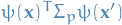 .
.
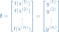
Predictions using noise-free observations
- We know

 = vector of training outputs
 = vector of test outputs
- Join distribution of training and test outputs according to the prior is then
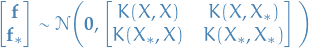 12
12
- If training points and
 test points, the matrix
 = covariaces evaluated at all pairs of training
and test points, and similarily for
= covariaces evaluated at all pairs of training
and test points, and similarily for  , etc.
 - Restrict this joint prior distribution to contain only
those functions which agree with the observed data points
- A lot of functions mate not efficient
In probabilistic terms this operation is simple: equivalent of conditioning on the joint Gaussian prior distribution on the observations to give
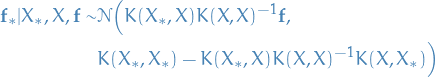 13
13
- A lot of functions mate
- Now we can sample values for
 (corresponding
to test inputs
(corresponding
to test inputs  ) from the joint posterior distribution
by evaluating the mean and covariance matrix from the eqn. above.
) from the joint posterior distribution
by evaluating the mean and covariance matrix from the eqn. above.
Appendix A: Stuff to know
Sampling from a Multivariate Gaussian
Assuming we have access to a Gaussian scalar generator.
Want samples  with arbitrary mean
  and covariance
  .
.
- Compute Cholesky decomposition (also known as "matrix square
root")
 of the positive (semi? not sure) definite symmetric
covariance matrix
of the positive (semi? not sure) definite symmetric
covariance matrix 
- is lower triangular matrix
- Generate
 by
multiple separate calls to the scalar Gaussian generator
by
multiple separate calls to the scalar Gaussian generator - Compute

- Has desired distribution with mean
 and covariance
![$L E[\mathbf{u}\mathbf{u}^T] L^T = LL^T = K$](../../assets/latex/gaussian_processes_for_machine_learning_395eba8336fdd19c8616bbbc9e617100b9536ec6.png) , by
independence of
, by
independence of 
- Has desired distribution with mean
Cholesky Decomposition
Decomposes a symmetric, positive definite matrix
 into
a product of a lower triangular matrix and its transpose:
into
a product of a lower triangular matrix and its transpose:
 14
14
- Useful for solving linear systems with symmetric, positive
definite coefficient matrix .
- Want to solve
 for
for 
- Solve the triangular system
 by forward substitution
 - Solve triangular system
 by backward substition
 - Solution is

 = vector which solves
- Want to solve
Complexity
- Both forward and backward substitution requires
 operations, when is of size
  .
. - The computation of the Cholesky factor is considered
numerically extremely stable and takes time
 .
.
Forward/backward substitution
For a lower triangular matrix we can write  as follows
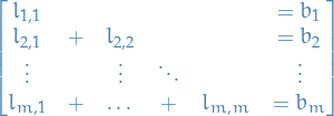 15
15
Notice that  , and so we can solve
 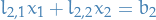 by substituting
  in, i.e. forward substitution.
Doing this repeatedly leads to the full solution for , that is:
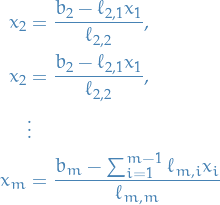 16
16
For backward substitution we do the exact same thing, just in reverse, since we're then dealing with a upper triangular matrix.
Appendix B: Derivations
Kernel
Declarations
 = input space
 = feature space
 = matrix with columns
  for all training inputs
Model
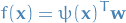 17
17
where is of length  . This is analogous to the standard linear model
except everywhere
. This is analogous to the standard linear model
except everywhere  is substituted for .
Appendix C: Exercises
Chapter 2: Regression
Ex. 1
First we import the stuff that needs to be imported
    %matplotlib inline
import numpy as np
import matplotlib.pyplot as plt
import seaborn as sns

    from __future__ import division
After having some issues, I found this article from which I used some of the code, so thanks a lot to Chris Fonnesbeck!
We start out by the following specification for our Gaussian Process:
 18
18
def exponential_cov(x, y, theta):
    return theta[0] * np.exp(-0.5 * theta[1] * np.subtract.outer(x, y) ** 2)
Then to compute the conditional probability for some new input conditioned on the previously send
inputs with outputs, we use the following:
 19
19
where, again, remember that and represents the test and training outputs, i.e in the case of
training (already seen) inputs:
 20
20
def conditional(X_star, X, y, theta):
    B = exponential_cov(X_star, X, theta)
    C = exponential_cov(X, X, theta)
    A = exponential_cov(X_star, X_star, theta)

    mu = np.linalg.inv(C).dot(B.T).T.dot(y)
    sigma = A - B.dot(np.linalg.inv(C).dot(B.T))

    return mu.squeeze(), sigma.squeeze()  # simply unwraps any 1-D arrays, so (1, 100) => (100,)
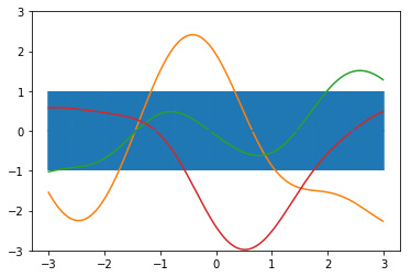
For now we set  :
:
theta = (1, 1)
sigma_theta = exponential_cov(0, 0, theta)
xpts = np.arange(-3, 3, step=0.01)
plt.errorbar(xpts, np.zeros(len(xpts)), yerr=sigma_theta, capsize=0)
    plt.ylim(-3, 3)

    # some sampled priors
    f1_prior = np.random.multivariate_normal(np.zeros(len(xpts)), exponential_cov(xpts, xpts, theta))
f2_prior = np.random.multivariate_normal(np.zeros(len(xpts)), exponential_cov(xpts, xpts, theta))
f3_prior = np.random.multivariate_normal(np.zeros(len(xpts)), exponential_cov(xpts, xpts, theta))
plt.plot(xpts, f1_prior)
plt.plot(xpts, f2_prior)
plt.plot(xpts, f3_prior)
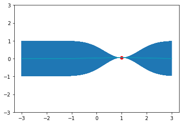
We select an arbitrary starting point, say  , and simply sample from a normal distribution
with unit covariance. This is just for us to have a "seen" sample to play with.
, and simply sample from a normal distribution
with unit covariance. This is just for us to have a "seen" sample to play with.
x = [1.]
y = [np.random.normal(scale=sigma_theta)]
np.array(y)
We now update our confidence band, given the point we just sampled,
by using the covariance function to generate new point-wise confidence intervals,
conditional on the value  seen above.
At a first glance it might look like conditional and predict_noiseless are the same functions,
but the difference is that predict_noiseless returns the mean and (noiseless) variance at each point
where as conditional returns the mean and the entire covariance matrix for all the test points.
So if you want to draw function samples (as we do later on), you'll want to use the conditional, while
if you're simply after the mean-line and it's uncertainty at each evaluated point you use the predict_noiseless.
sigma_1 = exponential_cov(x, x, theta)  # compute covariance for new point

def predict_noiseless(x, data, kernel, theta, sigma, f):
    K = [kernel(x, y, theta) for y in data]           # covariance between test input and training input
    sigma_inv = np.linalg.inv(sigma)                      # inverting the covariance matrix for training input
    K_dot_sigma_inv = np.dot(K, sigma_inv)
    y_pred = K_dot_sigma_inv.dot(f)                   # compute the predicted mean
    sigma_new = kernel(x, x, theta) - K_dot_sigma_inv.dot(K)  # covariance of new point

    return y_pred, sigma_new

x_pred = np.linspace(-3, 3, 2000)
predictions = [predict_noiseless(i, x, exponential_cov, theta, sigma_1, y) for i in x_pred]
y_pred, sigmas = np.transpose(predictions)
plt.errorbar(x_pred, y_pred, yerr=sigmas, capsize=0, alpha=0.6)
plt.plot(x, y, "ro")
plt.plot(x_pred, y_pred, c="c")
plt.ylim(-3, 3)
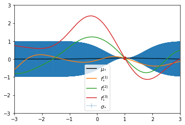
Notice that here we are predicting a mean and covariance  at each test point,
but for fun's sake we can sample some functions too!
at each test point,
but for fun's sake we can sample some functions too!
 21
21
That is; we create a normal distribution of dimension equal to the number of test inputs,
draw from this distribution, then the sample at index i corresponds to  , yah see?
It's weird, yes, but allows the indexed sample points to be any real value!
, yah see?
It's weird, yes, but allows the indexed sample points to be any real value!
    # same as above
plt.errorbar(x_pred, y_pred, yerr=sigmas, capsize=0, alpha=0.3, label="$\sigma_*$")
plt.plot(x, y, "ro")
plt.plot(x_pred, y_pred, c="black", label="$\mu_*$")
plt.ylim(-3, 3)
    plt.xlim(-3, 3)

# Some sampled functions
mu_star, K_star = conditional(x_pred, x, y, theta)       # x_pred conditioned on training input (x, y)
f1 = np.random.multivariate_normal(mu_star, K_star)
f2 = np.random.multivariate_normal(mu_star, K_star)
f3 = np.random.multivariate_normal(mu_star, K_star)
plt.plot(x_pred, f1, label="$f_*^{(1)}$")
plt.plot(x_pred, f2, label="$f_*^{(2)}$")
plt.plot(x_pred, f3, label="$f_*^{(3)}$")
    plt.legend()
Issues
I had multiple issues with following the book:
- Covariance matrix of the input matrix that I come up with
is not positive definite => can't use Cholesky decomposition
to draw samples, nor to circumvent having to compute the inverse.
There is no guarantee for this to be the case either, but there is a
guarantee that for a real matrix we will have a semi-positive definite
covariance matrix, which allows for drawing from a Gaussian by basically
replacing each L step with the equivalent SVD step (where we use the
product
 instead of ).
 - What to transpose and so on in the computation of the mean vector and covariance matrix for the predictions I got wrong multiple times… IT'S HARD, MKAY?!
Some of my own deprecated / horrible work
To generate samples  with arbitrary
mean and covariance matrix using a scalar Gaussian generator,
we proceed as follows:
with arbitrary
mean and covariance matrix using a scalar Gaussian generator,
we proceed as follows:
- Compute the Cholesky decomposition (also known as the "matrix square root") of the
positive-definite symmetric covariance matrix
 , where is lower triangular.
 - Generate by multiple separate calls to the scalar Gaussian generator.
- Compute , which has the desired distribution with:
- Mean
- Cov.
![$L \mathcal(E)[\mathbf{u}\mathbf{u}^T] L^T = LL^T = K$](../../assets/latex/gaussian_processes_for_machine_learning_c100167709245a0e426742f1336da32d40343e04.png) (by independence of the elements of )
(by independence of the elements of )
- Mean
def gaussian_draws(m, K, N=10000):
    """
    IMPORTANT: This version uses the Cholesky decomposition which ONLY works if the
    matrix `X` is positive definite symmetric, which is often not the case! A covariance
    matrix is only guaranteed to be SEMI-positive definite symmetric.
    """
    dim = m.shape[0]
    X = np.zeros((N, dim))

    L = np.linalg.cholesky(K)

    for i in range(N):
        u = np.random.normal(0, 1, dim)
        X[i, :] = m + np.dot(L, u)

    if N == 1:
        return X[0]  # return a single vector if only 1 sample is requested
    else:
        return X

m = np.array([2, 1, 0])
K = np.array([[2, -1, 0], [-1, 2, -1], [0, -1, 2]])  # this is positive-definite

X = gaussian_draws(m, K, 10)
X
Of course I could just have take advantage of the fact that numpy can generate the
entire sample-matrix for me, buuut I dunno, felt like doing some work myself, though
it's not much.
And if you want to know how we can draw from a semi-positive definite symmetric matrix, checkout this. Explains how you ought to use SVD in this case.
And then we need to able to compute the squared exponential kernel function:
 22
22
def squared_exponential(X, l=2):
    """
            DEPRECATED. Use exponential_cov instead. Much better.

    Computes the squared exponential (also known as Radial Basis function) of the
    the matrix `X`.

    Assumes `X` to be of the shape (n, p) where n is the number of samples, and p is the
    number of random variables for which we have samples.
    """
    dim = X.shape[0]
    K = np.zeros((dim, dim))

    for p in range(dim):
        x_p = X[p]

        for q in range(p, dim):
            x_q = X[q]
            diff = np.subtract(x_p, x_q)

            # since the resulting covariance matrix will be symmetric we only need to compute
            # the triangular matrix, and then copy the values.
            se = np.exp(- (1 / l) * (diff ** 2).sum())
            K[p, q] = se
            # stop us from assigning to the diagonal entries
            # twice, being SLIGHTLY more performant, yey!
            if p != q:
                K[q, p] = se


    return K

squared_exponential(np.arange(3))
Ex. 2
Bibliography
Bibliography
- [rasmussen2006gaussian] Rasmussen & Williams, Gaussian Processes for Machine Learning, MIT Press (2006).