Bandits
Table of Contents
Sequential decision problems
- Reward/feedback type:
- Bandit
- Only observe information/feedback for the action taken.
- Full information
- Observe information/feedback for all the actions.
- Partial information
- Observe information/feedback for a subset (potentially sparse) of possible actions.
- Bandit
Bandit book lattimore2018bandit
Notation
 denotes a stochastic bandit
 is the suboptimality gap or action gap or immediate regret of action
Number of times action
was chosen by the learner at the end of round 
In general, this is random, since the action taken at time
 is a random variable depending on all previous observatiosn and actions.
2
2.2 σ-algebras and knowledge
- Collection of sequential observations (rvs.)

- The set of maps
 such that
  is measurable then characterizes all the possible ways the learner can respond.
- I.e. sufficies to concentrate on σ-algebra

- I.e. sufficies to concentrate on σ-algebra
- Reminder:
 is adapted to filtration
  if
if  is
is  for each
 ![$t \in [n]$](../../assets/latex/bandits_77df7d259c970698dfceec77a36c5d52eec43d96.png) .
.
3
Markov Chains

4
4.5 Decomposing regret
For any policy  and stochastic bandit environment
  with
with  finite or countable and horizon
  , the regret
  of policy in satisfies
![\begin{equation*}
R_n = \sum_{a \in \mathcal{A}}^{} \Delta_a \mathbb{E} \big[ T_a(n) \big]
\end{equation*}](../../assets/latex/bandits_fffc6ec67a5bb6da46d3d3caae7a9dc5bc42573d.png)
5.
Exercises
5.3
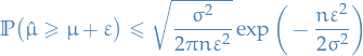
Eq. (5.2):
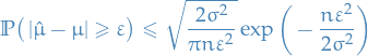
Eq. (5.4):
which means
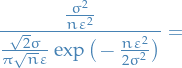
Then the ratio between the two rates:
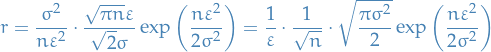
Then if  , we have
  and
and  is dominated by
Alternatively,
then

so,

As a result, on  the lower-bound of the ratio is monotonically increasing in
  . On
. On  , the lower-bound of the ratio decreases monotonically in . For the increase, we can for certain say that
We know for , the  factor completely dominates. For , we can use the fact that
which means that
But for the question of when  , i.e. Eq. (5.2) is best, and
  , i.e. Eq. (5.4) is best, observe that if
which means Eq. (5.4) is best (BUT,  so it doesn't actually provide us with any more information!).
Moreover, in the case  , we know for certain that
  and thus Eq. (5.4) is the best.
We can refine our lower-bound of when by using the slightly tighter lower-bound for , where we have
and we can solve for RHS = 1, or equiv.,
which is equivalent to the quadratic
which has solutions
Therefore has non-real imaginary component, i.e. this doesn't provide us with any more insight.
But, we can consider when this quadratic is  and
and  which gives us
6. The Explore-then-Commit Algorithm
Exercises
6.1 subGaussian empirical estimates
Let be the policy of ETC and  be the 1-subGaussian distributions associated with the
  arms.
arms.
Provide a fully rigorous proof of the claim that

is  . You should only use the definitions and the interaction protocol, which states that


Recall that
The mean reward for arm
 is estimated as
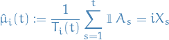
where
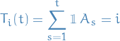
is the number of times action
has been played after round .
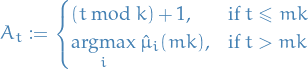
The ETC policy for parameter
 , which we denote
  , is defined by
First we note that is sufficient to show that  is
is  for all and that they're independent, since we can decompose the expression as:

and by Lemma 5.4 (c) (which we need to prove!) a sum of two subGaussian rvs is a subGaussian [Easy to prove though (Y)]
[I guess we need the interaction protocol to actually prove that we can consider the mean-estimates as independent?]
7. The Upper Condience Bound (UCB) Algorithm
Notation
Optimism principle
11. The Exp3 Algorithm
Notation
Conditional expectation given history up to time
![\begin{equation*}
E_t \big[ \wc \big] = \mathbb{E} \big[ \wc \mid A_1, X_1, \dots, A_{t - 1}, X_{t - 1} \big]
\end{equation*}](../../assets/latex/bandits_65419dea819ca839a60d74491c76968d5880acc3.png)
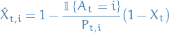
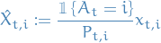
IS estimator of
 is
is
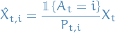
which satisfies
![\begin{equation*}
\mathbb{E}_t \big[ \hat{X}_{t, i} \big] = x_{t, i}
\end{equation*}](../../assets/latex/bandits_46ea048e1ee50e15245aa020ebfa980d67d9805f.png)
i.e. unbiased estimator. Note that in this case

Alternative (unbiased) estimator
which is more easily seen by rearranging
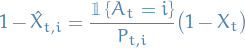
i.e. RHS is an estimate of the "loss"
 . Note that in this case
![\begin{equation*}
\hat{X}_{t, i} \in (-\infty, 1]
\end{equation*}](../../assets/latex/bandits_1b2fab581cb99f3c0a6eb96ae27c59d6a15de7d3.png)
Overview
- Adverserial bandits
11.3 The Exp3 algorithm
- Exp3 = Exponential-weight algorihtm for Exploration and Exploitation
- The idea is to construct unbiased estimators for the rewards from each arm by the use of IS.
Exp3 is a particular way of obtaining a distribution for each arm
at time ,  :
:
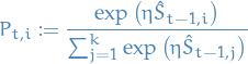
where
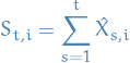
where
where
is the reward at time-step chosen for arm by the adversary.
 is referred to as the learning rate
- In simple case will be chosen depending on number of arms and horizon

- In simple case will be chosen depending on number of arms
Let
![$x \in [0, 1]^{n \times k}$](../../assets/latex/bandits_0db521f5aa07e1b7146ac31f6ce53e70147c77d8.png)
- be the policy of
Exp3with learning rate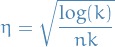
Then
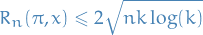
For any arm define
![\begin{equation*}
R_{n, i} = \sum_{t = 1}^{n} x_{t, i} - \mathbb{E} \bigg[ \sum_{t = 1}^{n} X_t \bigg]
\end{equation*}](../../assets/latex/bandits_4e2a8f7e1755bc84bda1f4f77dab7dd6c0370fd0.png)
which is the expected regret relative to using action in all the rounds.
We will bound  for all , including the optimal arm.
18. Contextual Bandits
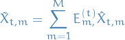
For any ![$m^{\ast} \in [M]$](../../assets/latex/bandits_8a1a7713b40dfe3bfe2522906ea47276f7efb2aa.png) , it holds that
, it holds that
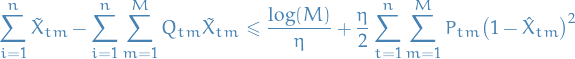
Recall that

i.e.
19. Linear Stochastic Bandits
19.3 Regret Analysis
Let  be positive definite and
  be a sequence of vectors with
  for all .
Then
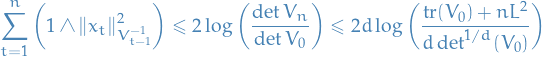
In the final inequality we have the following argument.
Operator norm of the matrix  is going to be bounded by
  , since
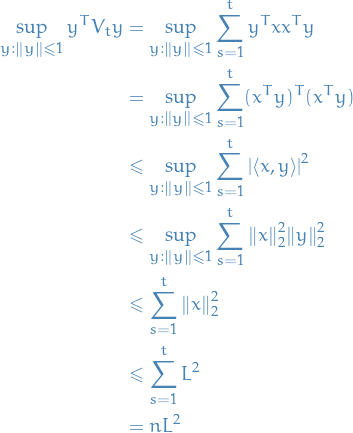
where in the third inequality we've made use of the Cauchy inequality and the assumption that  .
.
The factor of 2 shows up because we do

and each of these terms are bounded by  due to the vectors being in
  .
.
20.
20.1
Errata
- p. 79: in point 3), there's a sum without any terms…
Linear bandits
Contextual bandits
Batched bandits
- han20_sequen_batch_learn_finit_action
- Analysis of both adverserial and stochastic contexts (both with stochastic rewards)
- Finite number of arms
- Number of batches
 is allowed to scale wrt.
  , and for the relevant results, they provide lower-bounds on the number of batches necessary to achieve the desired regret.
 - Analysis is done by analysing the prediction error of a linear regression model which has seen
 observations, where
  is the index of the batch. From this we can deduce the regret of following the predictions based on these previous observations rather than the online version.
 - Algorithm presented is essentially LinUCB?
- Adverserial contexts
Lower-bound on the regret of any sequential batched algoritm for the case of
 han20_sequen_batch_learn_finit_action
![\begin{equation*}
\sup_{\theta^{\ast}: \norm{\theta^{\ast}}_2 \le 1} \mathbb{E} \big[ R_T(\mathrm{Alg}) \big] \ge c \cdot \Bigg( \sqrt{d T} + \bigg( \frac{T \sqrt{d}}{M} \land \frac{T}{\sqrt{M}} \bigg) \Bigg)
\end{equation*}](../../assets/latex/bandits_3a4463e0017040596f4cda75f6cf1214efb45b9c.png)
where
 is the number of arms
 is dimensionality of
Reward is modelled as

where
 .
.
- is horizon
- is number of batches
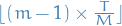
 denotes the algorithm which consists of a "time-grid"
  (with each "interval" in the grid corresponding to a single batch, so that
  ) and the learning algorithm/policy which maps previous observations to next action to take.
 is a universal constant independent of
- Stochastic contexts
- Upper-bound on regret for what's essentially LinUCB han20_sequen_batch_learn_finit_action