Approximate Bayesian Computation (ABC)
Table of Contents
Notation
 parameters
 generated samples from model with parameters
 denotes observed data
 is the domain of the observations
 is a metric on
Overview
- Cases where computing the likelihood of the observed data is intractable
- ABC uses approximation of the likelihood obtained from simulation
Rejection ABC
Let  be a similarity threshold, and be the notion of distance, e.g. premetric on domain of observations.
The rejection ABC proceeds as follows:
- Sample multiple model parameters
 .
. - For each , generate psuedo-dataset
 from
from - For each psuedo-datset , if
 , accept the generated , otherwise reject .
Result: Exact sample  from approximated posterior
  , where

Choice of is crucial in the design of a n accurate ABC algorithm.
Soft ABC
One can interpret the approximate likelihood  in rejection ABC as the convolution of the true likelihood and the "similarity" kernel

In fact, one can use any similarity kernel parametrised by  satisfying

which gives rise to the Soft ABC methods:
Soft ABC is an extension of rejection ABC which instead weights the parameter samples from the model instead of rejecting or accepting.
An example is using the Gaussian kernel:
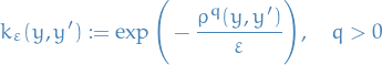
Which results in the weighted sample
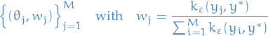
which can be directly utilized in estimating posterior expectations, i.e. for a test function 
![\begin{equation*}
\mathbb{\hat{E}} \big[ f(\theta) \big] = \sum_{i=1}^{M} w_j f(\theta_j)
\end{equation*}](../../assets/latex/approximate_bayesian_computation_fb1a65361822bd3a8a9eb9d66fb374dcf23af647.png)