Options
Table of Contents
Notation
- call option: buyer / owner of the option has the right to buy
- put option: buyer / owner of the option has the right to sell
- strike price or exercise price: the pixed price at which the owner of the option can buy (in call), or sell (in put) the underlying security or commodity
- call (put) is in-the-money if the strike price is below (above) the market price
- call (put) is out-of-the-money if the strike price is above (below) the market price
Option-styles
The style or family of an option is the class into which the option falls, usually defined by the dates on which the option may be exercised.
The vast majority of options are either European or American (style) options.
The key differences between American and European options relates to when the options can be exercised:
- European option may be exercised only at the expiration date of the option, i.e. at a single pre-defined point in time.
- American option may be exercised at any time before the expiration date.
Pricing
Black-Scholes
- Model for dynamics of financial market containing derivative investment instruments
- Key idea: hedge the option by buying and selling the underlying asset in the just the right away, thus eliminate risk
Notation
 is the price of the stock
 the price of a derivative as a function of time and stock price
 the price of a European call option
 the price of a European put option
 the strike price of the option
 the annualized risk-free interest rate, continuously compounded
 the drift rate of , annualized
 the std. dev. of stock's returns
 a time in years with
  being the expiry
- $Π the value of the portfolio
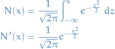
 denotes the /std. normal cumulative distribution function, and
  the std. normal density:
Assumptions
Assumptions on the underlying assets:
- Riskeless rate: rate of return on the riskless asset is constant and thus called the risk-free interest rate
- Random walk: instantaneous log return of the stock price is infinitesimal random walk with drift; it's a geometric Brownian motion, and we will assume its drift and volatility are constant
- If time-varying, one can deduce a modified Black-Scholes formula, as long as the volatility is not random
- Stock does not pay dividends
Assumptions on the market:
- No arbitrage
- Possible to borrow and lend any amount, even fractional, of cash at a riskless rate
- Possible ot buy and sell any amount, even fractional, of the stock (includes short-selling)
- Above transactions do not incur any fees or costs (i.e. frictionless market)
The Black-Scholes equation is a partial differential equation, which describes the price of the option over time:
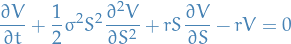
- Gives a theoretical estimate of the price of European-style options, and shows that it has a unique price regardless of the risk of the security and its expected return
Shorting
Shorting a stock refers to the following:
- You sell
 stocks at some price
  without actually owning these stocks
- Behind the scenes, the exchange-provider or whatever borrows stocks from someone in the following sense:
- Provider obtains stocks from a current owner of the company
- Provider gives the obtained stocks to the purchaser of your "imaginary" sell
- Provider obtains
- Thus, as long as the short-position is "open", the agent which the provider "borrowed" stocks have "technically" lost their stocks, but know that you will have to buy stocks back to them at some point
- Behind the scenes, the exchange-provider or whatever borrows
- At a later stage, you buy back stocks at some price

- These stocks are then given to the provider, which in turn gives the stocks to the agent of which the provider obtained the original stocks that were sold at the beginning
You, as the shorter, is then left with the following profit:  .
.
The outcomes are then:
 , i.e. the stock increased in value while you "borrowed" the stock (had the short-position) and you lost
  , i.e. the stock decreased in value while you "borrowed" the stock (had the short-position) and you /earned7
Huge caveats:
- The original owner of the stocks usually have the right to reclaim the stocks whenever they want, in which case your short-position will be closed immediately, i.e. the price will be whatever the current price is.
- As a result, if you hypothesize that the stocks will decrease in value tomorrow and so you short today, there's a non-zero probability of you having to close the position today!
- Worth noting that the orignal owner doesn't know anything about who is borrowing their stocks, so it's not possible for someone to specifically target you by first providing stocks to your short-position and then reclaiming them as soon as there's an increase in the stock's price
- BUT short-positions are generally available to the public (at least on OSEBX), so there's definitively a chance that if someone wants to see the world burn can just start reclaiming all their stocks arbitrarily
- At the same time, if you keep your short-position open for a period of time, there's usually a "borrowing fee" involved which is due every, say, day of borrowing. Therefore, it's usually beneficial for the original owner of the stock to allow you to borrow as long as you want.
- As a result, if you hypothesize that the stocks will decrease in value tomorrow and so you short today, there's a non-zero probability of you having to close the position today!