Term rewriting
Table of Contents
Notation
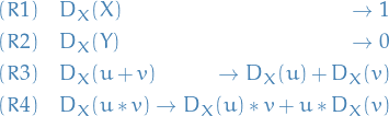
 denotes rewrite rule which rewrites
  to
to  , but not the other way around
Preface
- Term rewriting vs. equational logic
- In term rewriting: equations are used as directed replacement rules, i.e. LHS can be replaced by RHS, but not vice versa
- Equational reasoning is concerned with a rather restricted class of first-order languages
- Only predicate symbol is equality
Motivating Examples
- Term rewriting system
- Terms are built up by
- variables
- constant symbols
- function symbols
- Termination: is it always the case that after finitely many rule applications we reach an expression to which no more rules apply?
- The resulting expression is called a normal form
Let  be a term.
The normal form of , denoted  , is a term s.t. no further rewrite rules are applicable.
Symbolic derivation
Consider rules
struct Termz{Op}
    args
end

struct D
    var
    expr
end

Termz(x) = x
Termz(expr::Expr) = begin
    @assert expr.head === :call
    Termz{eval(expr.args[1])}(Termz.(expr.args[2:end]))
end

terms(op, args::AbstractArray) = length(args) > 1 ? Termz{op}(args) : args[1]

# Have to implement this explicitly since using different arrays to hold `args`
import Base: ==
==(t1::Termz{Op1}, t2::Termz{Op2}) where {Op1, Op2} = false
==(t1::Termz{Op}, t2::Termz{Op}) where Op = (t1.args ∩ t2.args) == t1.args

t = Termz(:(3x + 2))

D(x, y::Termz) = Termz{D}([x, y])
D(x::Termz, y::Termz) = x == y ? 1 : Termz{D}([x, y])
D(x::Symbol, y::Symbol) = x == y ? 1 : 0
D(x, y::Number) = 0
D(x, t::Termz{+}) = begin
    # @info "calling Termz{+} with args" t

    Termz{+}(D.(x, t.args))
end
D(x, t::Termz{*}) = begin
    # @info "calling Termz{*} with args" t

    Termz{+}([
        Termz{*}([ D(x, t.args[1]), t.args[2:end]... ]),
        Termz{*}([ t.args[1], D(x, terms(*, t.args[2:end])) ])
    ])
end
D(x, t::Termz{^}) = begin
    # @info "calling Termz{^} with args" t

    Termz{*}([
        t.args[end], # exponent
        Termz{^}([
            t.args[1],
            Termz{+}([t.args[end], -1])
        ])
    ])
end

eval(x::Number) = x
eval(x::Number, dict) = x
eval(x::Symbol, dict) = dict[x]
eval(t::Termz{Op}) where Op = foldl(Op, eval.(t.args))
eval(t::Termz{Op}, dict) where Op = foldl(Op, [eval(a, dict) for a ∈ t.args])
(t::Termz)(; kwargs...) = eval(t, kwargs)

function variables(t::Termz; res = Set())
    for t_ ∈ t.args
        if t_ isa Symbol
            push!(res, t_)
        elseif t_ isa Termz
            variables(t_; res = res)
        end
    end

    return res
end


"Generates an anonymous function which evaluates together with the variable ordering."
generate(t::Termz) = begin
    vars = collect(variables(t))

    if length(vars) == 0
        return () -> eval(t, Dict()), []
    end

    expr = quote
        ($(vars...)) -> eval(t, Dict(zip($vars, [$(vars...)])))
    end

    return eval(expr), vars
end


# TESTING

eval(D(:x, t), Dict(:x => 2.0))

eval(t, Dict(:x => 1.0))

der = D(:x, Termz(:(3 * x * y)))
der(; x = 0.0, y = 1.0)

# Addition
t = Termz(:(x + 1))
@assert t(; x = 1) == 2
@assert D(:x, t)(; x = 100) == 1

# Multiplication
t = Termz(:(x * y))
@assert t(; x = 1.0, y = 2.0) == 2.0
@assert D(:x, t)(; x = 1.0, y = 2.0) == 2.0

# Power
t = Termz(:(x^3))
@assert t(; x = 2.0) == 8.0
@assert D(:x, t)(; x = 2.0) == 12.0

# All combined
t = Termz(:((3 + x)x^2 + 2x + 1))
@assert t(; x = 1) == 7
@assert D(:x, t)(; x = 2) == 26

println(D(:x, t))
println(D(:x, t)(; x = 2))

println(D(:x, Termz(:(x * x))))

# Macros for convenience

macro termz(expr)
    Termz(expr)
end

macro D(var, expr)
    D(Termz(var), Termz(expr))
end

println()
println("Macros:")
println(@termz 1 + x)
println(@D(x, 1 + 100x))
println(@D(x, x * x))


println(@D(x, f(x)))
println(D(:x, @termz f(x)))
println(@D(f(x), f(x)))
# println(@D(g(x), f(x)))  # FIXME: currently requires the function to be defined

g() = 1  # but doesn't have to have the correct signature; though `eval` will fail
println(@D(g(x), f(x)))
Termz{+}(Any[Termz{+}(Termz{*}[Termz{*}(Termz[Termz{+}([0, 1]), Termz{^}(Any[:x, 2])]), Termz{*}(Termz[Termz{+}(Any[3, :x]), Termz{*}(Any[2, Termz{^}(Any[:x, Termz{+}([2, -1])])])])]), Termz{+}(Termz{*}[Termz{*}(Any[0, :x]), Termz{*}([2, 1])]), 0])
26
Termz{+}(Termz{*}[Termz{*}(Any[1, :x]), Termz{*}(Any[:x, 1])])

Macros:
Termz{+}(Any[1, :x])
Termz{+}(Any[0, Termz{+}(Termz{*}[Termz{*}(Any[0, :x]), Termz{*}([100, 1])])])
Termz{+}(Termz{*}[Termz{*}(Any[1, :x]), Termz{*}(Any[:x, 1])])
Termz{D}(Any[:x, Termz{f}(Symbol[:x])])
Termz{D}(Any[:x, Termz{f}(Symbol[:x])])
1
Termz{D}(Termz[Termz{g}(Symbol[:x]), Termz{f}(Symbol[:x])])
By applying the corresponding rules in sequence we get

- Confluence
- Say there are different ways of applying rules to a given term
- Suppose these different ways lead to two different terms
 and
and 
- Can we always find a common term
 that can be reached from both and by application of the defined rules?
 - If this is true (for all terms in this system), we have confluence for the defined rules
- Say there are different ways of applying rules to a given term
- Completion
- Can we always make a non-confluent system into a confluent system by adding implied rules
- This is referred to as completion of the system
One can show that  is actually confluent.
- Suppose we have some arbitrary term
- Consider all possible rules that was applied to the previous term

OR
- All rules are independent
- Rules constitutes a functional program
- On the LHS, the defined function
 occurs only at the very outside
- On the LHS, the defined function
- Termination of the resul means that $DX is a total function
- Confluence of the rules means that the result of a computation is independent of the evaluation/rewrite strategy
All term rewriting systems that constitute functional programs are confluent.
Group Theory
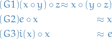
Given a set of identities  and two terms and , is it possible to transform the term into the term , using the identities in as rewrite rules that can be applied in both directions?
There are a couple of problems we need to overcome:
- Equivalent terms can have distinct normal forms
- Normal forms need not exist
Abstract reduction system
An abstract reduction system is a pair  , where the reduction
  is a binary relation on the set
  , i.e.
  .
.
Instead of  we write
  ..
..
So a binary relation is just a subset of  which satisfy some property.
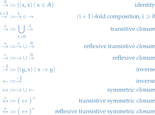
Notation
Identity:

(i + 1)-fold composition,


Transistive closure

Reflexive transistive closure

Reflexive closure

Inverse

Inverse

Symmetric closure

Transistive symmetric closure

Reflexive transistive symmetric closure

- is reducible if and only if

- is in normal form (irreducible) if and only if it is not reducible
- is a normal form of if and only if
 and is in normal form. If has a uniquely determined normal form, the latter is denoted by
  .
. - is a direct successor of if and only if
- is a successor of if and only if

- and are joinable if and only if

in which case we write

A reduction
is called Church-Rosser if and only if

A reduction
is called confluent if and only if

- A reduction is called terminating if and only if there is no infinitiely descending chain

- A reduction is called normalizing if and only if every element has a normal form
- A reduction is called convergent if and only if it is both confluent and terminating
Equivalence and reduction
Can view reduction in two ways
- Directed computation, starting from some point
 , and then tries to reac a normal form by following the reduction
- Corresponds to idea of program evaluation
- Consider merely as a description of
 , where
  means that there is a path between
  and
and  where the arrows can be traversed in both directions, e.g.
- Corresponds to idea of identities which can be used in both directions
So
- (2) is of course very slow to do in general, so would be nice if we could do (1) until we reach normal form and then compare the normal forms of the expressions
- Only works if reduction terminates and normal forms are unique: formally, we need termination and confluence of reduction
Basic definitions
- Two relations
 and
and 
Their composition is defined by

- Notations like
 and
and  only work for arrow-like symbols
- In the case of arbitrary relations
 we write
  , etc.
- In the case of arbitrary relations
- Some of the constructions can also be expressed nicely in terms of paths:
 if there is a path of length
  from to
 - if there is some finite path from to
 if there is some finite nonempty path from to
- The
 of
of  is the least set with property
  which contains
- E.g.
 , the reflexive transistive closure of , is the least reflexive and transisitve relation which contains .
 - For arbitrary and , the of need not exist, but in the above cases they always do because reflexivity, transistivity and symmetry are closed under arbitrary intersections
- In such cases, the can be be defined directly as the intersection of all sets with property which contain
- In such cases, the
- E.g.
- Claim: is the least equivalence relation containing
- Proof: An equivalence relation containing must also contain by the symmetry property of a equivalence relation, thus is contains
 . We just need to verify that it also contains
  and any number of . Observe first that
  is definitively in it because of the reflexitivity of the equivalence relation. Finally it then contains
  because of transistivity. Hence any other equivalence relation
  containing must contain (set corresponding to ), i.e. it's the least equivalence relation containing .
- Proof: An equivalence relation containing
Sudoku solver
- Why? Because we can
cell_candidates(i, j, grid) = [k for k = 1:size(grid, 1) if k ∉ (Set(grid[i, :]) ∪ Set(grid[:, j]))]

subsolve!(grid) = begin
    # solve all the straight forward ones
    for i = 1:size(grid, 1)
        for j = 1:size(grid, 2)
            if grid[i, j] == 0
                candidates = cell_candidates(i, j, grid)
                if length(candidates) == 1
                    grid[i, j] = candidates[1]
                end
            end
        end
    end

    grid
end

solve!(grid; level = 0) = begin
    @info level

    success = false
    prev_soln = zeros(size(grid))

    num_steps = 0
    while grid != prev_soln
        copy!(prev_soln, grid)
        subsolve!(grid)

        # increment step counter
        num_steps += 1
        # @info "Completed step $num_steps"
    end

    # at this point, we either solved it completely or there are ambigious entries
    unsolved = findall(zeros(size(grid)) .== grid)
    # @info "unsolved" unsolved
    issolved = length(unsolved) == 0
    if !issolved
        # try out filling in different entries; starting with the ones with the fewest
        # possible candidates
        unsolved_ns = [length(cell_candidates(idx[1], idx[2], grid)) for idx ∈ unsolved]
        if 0 ∈ unsolved_ns
            return false
        end

        unsolved_indices = sort(1:length(unsolved); by = i -> unsolved_ns[i])
        # @info unsolved_ns[unsolved_indices]

        for i ∈ unsolved_indices
            idx = unsolved[i]
            soln = copy(grid)

            for v ∈ cell_candidates(idx[1], idx[2], soln)
                soln[idx] = v
                issolved = solve!(soln; level = level + 1)
                issolved && @info soln
                if issolved
                    grid .= soln
                    return true
                end
            end

            # @info "failed to solve grid"
        end
    end

    unsolved = findall(zeros(size(grid)) .== grid)
    return length(unsolved) == 0 # issolved
end

solve(grid) = begin
    soln = copy(grid)
    issolved = solve!(soln)
    if !issolved
        @warn "failed to solve Sudoku"
    end

    return soln
end

# # simple case
# grid = [
#     0 1 3;
#     3 2 0;
#     0 0 2
# ]
# @assert solve(grid) == [2 1 3; 3 2 1; 1 3 2]

# grid = [
#     0 1 3 0 5;
#     3 2 0 0 0;
#     0 0 2 0 0;
#     4 0 0 3 0;
#     1 0 0 0 0
# ]

# solve(grid)

# FAILED!!!
# Takes forever to run; might be a mistake in the grid
grid = [
    5 3 0 0 7 0 0 0 0;
    6 0 0 1 9 6 0 0 0;
    0 9 8 0 0 0 0 6 0;
    8 0 0 0 6 0 0 0 3;
    4 0 0 8 0 3 0 0 1;
    7 0 0 0 2 0 0 0 6;
    0 6 0 0 0 0 2 8 0;
    0 0 0 4 1 9 0 0 5;
    0 0 0 0 8 0 0 7 9;
]
size(grid)
@time res = solve(grid)

# Solved ✓
# - Requires 1 lvl nesting
grid = [
    0 0 3 0 1 0;
    5 6 0 3 2 0;
    0 5 4 2 0 3;
    2 0 6 4 5 0;
    0 1 2 0 4 5;
    0 4 0 1 0 0;
]

# Solved ✓
# - Requires 4 lvl nesting
grid = [
    0 0 0 1 0 6;
    6 0 4 0 0 0;
    1 0 2 0 0 0;
    0 0 0 5 0 1;
    0 0 0 6 0 3;
    5 0 6 0 0 0;
]

# Solved ✓
# - Requires 14 lvl nesting
grid = [
    0 0 0 4 0 0;
    0 0 6 0 0 3;
    0 0 0 0 0 0;
    0 0 0 0 0 0;
    6 0 0 5 0 0;
    0 0 1 0 0 0
]

# 7 x 7
# Solved ✓
# - Requires 17 lvl nesting
grid = [
    0 4 0 0 3 1 6 0;
    1 0 0 0 0 0 0 0;
    8 0 0 0 0 0 0 0;
    4 3 0 0 2 0 0 0;
    0 0 0 8 0 0 3 4;
    0 0 0 0 0 0 0 5;
    0 0 0 0 0 0 0 6;
    0 7 4 5 0 0 8 0;
]

# 8 x 8
# Solved ✓
# - Requires 10 lvl nesting
grid = [
    0 0 0 0 7 0 0 6;
    0 0 0 5 3 0 0 7;
    0 0 0 0 0 6 1 0;
    3 0 2 0 0 5 0 0;
    0 0 0 0 0 0 0 1;
    8 4 0 0 0 0 0 0;
    0 0 8 0 0 2 0 0;
    0 6 0 1 5 0 0 0
]

# Solved ✓
# - Requires lvl 14 nesting
grid = [
    0 0 0 2 0 3 0 0;
    0 0 6 0 0 7 0 0;
    3 8 0 0 0 0 6 0;
    0 0 0 7 3 0 0 5;
    7 0 0 4 1 0 0 0;
    0 2 0 0 0 0 7 4;
    0 0 3 0 0 5 0 0;
    0 0 1 0 7 0 0 0;
]
@assert size(grid) == (8, 8)

# 9 x 9
# Solved ✓
# - Requires lvl 14 nesting
# - @time: 1.177324 seconds (16.63 M allocations: 1.678 GiB, 17.42% gc time)
grid = [
    5 3 0 0 7 0 0 0 0;
    6 0 0 1 9 5 0 0 0;
    0 9 8 0 0 0 0 6 0;
    8 0 0 0 6 0 0 0 3;
    4 0 0 8 0 3 0 0 1;
    7 0 0 0 2 0 0 0 6;
    0 6 0 0 0 0 2 8 0;
    0 0 0 4 1 9 0 0 5;
    0 0 0 0 8 0 0 7 9
]

# Solved ✓
# - Requires lvl 18 nesting
# - @time: 0.020624 seconds (285.23 k allocations: 28.252 MiB, 11.97% gc time)
grid = [
    0 0 0 1 0 5 0 6 8;
    0 0 0 0 0 0 7 0 1;
    9 0 1 0 0 0 0 3 0;
    0 0 7 0 2 6 0 0 0;
    5 0 0 0 0 0 0 0 3;
    0 0 0 8 7 0 4 0 0;
    0 3 0 0 0 0 8 0 5;
    1 0 5 0 0 0 0 0 0;
    7 9 0 4 0 1 0 0 0;
]

# Solved ✓
# - Requires lvl 39 nesting
# - @time: 0.036620 seconds (693.66 k allocations: 68.903 MiB, 16.69% gc time)
grid = [
    1 0 0 0 0 0 0 0 0;
    0 0 0 0 1 2 0 0 0;
    0 0 0 0 0 0 0 0 1;
    0 8 0 0 0 0 5 0 1;
    0 5 0 0 8 9 0 0 7;
    0 9 0 0 0 0 0 0 0;
    0 0 0 0 0 0 6 5 0;
    0 0 0 0 0 0 0 0 0;
    0 0 0 0 3 0 0 0 0;
]

# Solved ✓
# - Requires 2 lvl nesting
# - @time: 0.011032 seconds (160.33 k allocations: 16.076 MiB, 20.82% gc time)
grid = [
    0 0 9 0 7 0 4 3 6;
    0 0 0 3 8 0 9 0 0;
    6 3 2 5 0 0 0 0 0;
    7 6 3 8 0 0 0 4 0;
    4 0 0 1 0 7 0 0 8;
    0 2 0 0 0 3 5 6 7;
    0 0 0 0 0 8 2 7 3;
    0 0 6 0 3 9 0 0 0;
    3 5 8 0 1 0 6 0 0;
]

@assert size(grid) == (9, 9)
@time res = solve(grid)
res